Quantum Machine Learning API using QPanda¶

Quantum Computing Layer¶

QuantumLayer¶

QuantumLayer is a package class of autograd module that supports ariational quantum circuits. You can define a function as an argument, such as qprog_with_measure, This function needs to contain the quantum circuit defined by pyQPanda: It generally contains coding-circuit, evolution-circuit and measurement-operation. This QuantumLayer class can be embedded into the hybrid quantum classical machine learning model and minimize the objective function or loss function of the hybrid quantum classical model through the classical gradient descent method. You can specify the gradient calculation method of quantum circuit parameters in QuantumLayer by change the parameter diff_method. QuantumLayer currently supports two methods, one is finite_diff and the other is parameter-shift methods.

The finite_diff method is one of the most traditional and common numerical methods for estimating function gradient.The main idea is to replace partial derivatives with differences:

\[f^{\prime}(x)=\lim _{h \rightarrow 0} \frac{f(x+h)-f(x)}{h}\]

For the parameter-shift method we use the objective function, such as:

\[O(\theta)=\left\langle 0\left|U^{\dagger}(\theta) H U(\theta)\right| 0\right\rangle\]

It is theoretically possible to calculate the gradient of parameters about Hamiltonian in a quantum circuit by the more precise method: parameter-shift.

\[\nabla O(\theta)= \frac{1}{2}\left[O\left(\theta+\frac{\pi}{2}\right)-O\left(\theta-\frac{\pi}{2}\right)\right]\]

class pyvqnet.qnn.quantumlayer.QuantumLayer(qprog_with_measure, para_num, machine_type_or_cloud_token, num_of_qubits: int, num_of_cbits: int = 1, diff_method: str = 'parameter_shift', delta: float = 0.01, dtype=None, name='')¶

Abstract calculation module for variational quantum circuits. It simulates a parameterized quantum circuit and gets the measurement result. QuantumLayer inherits from Module ,so that it can calculate gradients of circuits parameters,and train variational quantum circuits model or embed variational quantum circuits into hybird quantum and classic model.

This class dos not need you to initialize virtual machine in the qprog_with_measure function.

Parameters:

qprog_with_measure – callable quantum circuits functions ,cosntructed by qpanda
para_num – int - Number of parameter
machine_type_or_cloud_token – qpanda machine type or pyQPANDA QCLOUD token : https://pyqpanda-toturial.readthedocs.io/zh/latest/Realchip.html
num_of_qubits – num of qubits
num_of_cbits – num of classic bits
diff_method – ‘parameter_shift’ or ‘finite_diff’
delta – delta for diff
dtype – The data type of the parameter, defaults: None, use the default data type kfloat32, which represents a 32-bit floating point number.
name – name of the output layer

Returns:

a module can calculate quantum circuits .

Note

qprog_with_measure is quantum circuits function defined in pyQPanda :https://pyqpanda-toturial.readthedocs.io/zh/latest/QCircuit.html.

This function should contain following parameters,otherwise it can not run properly in QuantumLayer.

qprog_with_measure (input,param,qubits,cbits,m_machine)

input: array_like input 1-dim classic data

param: array_like input 1-dim quantum circuit’s parameters

qubits: qubits allocated by QuantumLayer

cbits: cbits allocated by QuantumLayer.if your circuits does not use cbits,you should also reserve this parameter.

m_machine: simulator created by QuantumLayer

Use the m_para attribute of QuantumLayer to get the training parameters of the variable quantum circuit. The parameter is a QTensor class, which can be converted into a numpy array using the to_numpy() interface.

Note

The class have alias: QpandaQCircuitVQCLayer .

Example:

import pyqpanda as pq
from pyvqnet.qnn.measure import ProbsMeasure
from pyvqnet.qnn.quantumlayer import QuantumLayer
import numpy as np
from pyvqnet.tensor import QTensor
def pqctest (input,param,qubits,cbits,m_machine):
    circuit = pq.QCircuit()
    circuit.insert(pq.H(qubits[0]))
    circuit.insert(pq.H(qubits[1]))
    circuit.insert(pq.H(qubits[2]))
    circuit.insert(pq.H(qubits[3]))

    circuit.insert(pq.RZ(qubits[0],input[0]))
    circuit.insert(pq.RZ(qubits[1],input[1]))
    circuit.insert(pq.RZ(qubits[2],input[2]))
    circuit.insert(pq.RZ(qubits[3],input[3]))

    circuit.insert(pq.CNOT(qubits[0],qubits[1]))
    circuit.insert(pq.RZ(qubits[1],param[0]))
    circuit.insert(pq.CNOT(qubits[0],qubits[1]))

    circuit.insert(pq.CNOT(qubits[1],qubits[2]))
    circuit.insert(pq.RZ(qubits[2],param[1]))
    circuit.insert(pq.CNOT(qubits[1],qubits[2]))

    circuit.insert(pq.CNOT(qubits[2],qubits[3]))
    circuit.insert(pq.RZ(qubits[3],param[2]))
    circuit.insert(pq.CNOT(qubits[2],qubits[3]))
    #print(circuit)

    prog = pq.QProg()
    prog.insert(circuit)
    # pauli_dict  = {'Z0 X1':10,'Y2':-0.543}
    rlt_prob = ProbsMeasure([0,2],prog,m_machine,qubits)
    return rlt_prob

pqc = QuantumLayer(pqctest,3,"cpu",4,1)
#classic data as input
input = QTensor([[1,2,3,4],[40,22,2,3],[33,3,25,2.0]] )
#forward circuits
rlt = pqc(input)
grad =  QTensor(np.ones(rlt.data.shape)*1000)
#backward circuits
rlt.backward(grad)
print(rlt)
# [
# [0.2500000, 0.2500000, 0.2500000, 0.2500000],
# [0.2500000, 0.2500000, 0.2500000, 0.2500000],
# [0.2500000, 0.2500000, 0.2500000, 0.2500000]
# ]

QuantumLayerV2¶

If you are more familiar with pyQPanda syntax, please using QuantumLayerV2 class, you can define the quantum circuits function by using qubits, cbits and machine, then take it as a argument qprog_with_measure of QuantumLayerV2.

class pyvqnet.qnn.quantumlayer.QuantumLayerV2(qprog_with_measure, para_num, diff_method: str = 'parameter_shift', delta: float = 0.01, dtype=None, name='')¶

Abstract calculation module for variational quantum circuits. It simulates a parameterized quantum circuit and gets the measurement result. QuantumLayer inherits from Module ,so that it can calculate gradients of circuits parameters,and train variational quantum circuits model or embed variational quantum circuits into hybird quantum and classic model.

To use this module, you need to create your quantum virtual machine and allocate qubits and cbits.

Parameters:

qprog_with_measure – callable quantum circuits functions ,cosntructed by qpanda
para_num – int - Number of parameter
diff_method – ‘parameter_shift’ or ‘finite_diff’
delta – delta for diff
dtype – The data type of the parameter, defaults: None, use the default data type kfloat32, which represents a 32-bit floating point number.
name – name of the output layer

Returns:

a module can calculate quantum circuits .

Note

qprog_with_measure is quantum circuits function defined in pyQPanda :https://pyqpanda-toturial.readthedocs.io/zh/latest/QCircuit.html.

This function should contains following parameters,otherwise it can not run properly in QuantumLayerV2.

Compare to QuantumLayer.you should allocate qubits and simulator: https://pyqpanda-toturial.readthedocs.io/zh/latest/QuantumMachine.html,

you may also need to allocate cbits if qprog_with_measure needs quantum measure: https://pyqpanda-toturial.readthedocs.io/zh/latest/Measure.html

qprog_with_measure (input,param)

input: array_like input 1-dim classic data

param: array_like input 1-dim quantum circuit’s parameters

Note

The class have alias: QpandaQCircuitVQCLayerLite .

Example:

import pyqpanda as pq
from pyvqnet.qnn.measure import ProbsMeasure
from pyvqnet.qnn.quantumlayer import QuantumLayerV2
import numpy as np
from pyvqnet.tensor import QTensor
def pqctest (input,param):
    num_of_qubits = 4

    m_machine = pq.CPUQVM()# outside
    m_machine.init_qvm()# outside
    qubits = m_machine.qAlloc_many(num_of_qubits)

    circuit = pq.QCircuit()
    circuit.insert(pq.H(qubits[0]))
    circuit.insert(pq.H(qubits[1]))
    circuit.insert(pq.H(qubits[2]))
    circuit.insert(pq.H(qubits[3]))

    circuit.insert(pq.RZ(qubits[0],input[0]))
    circuit.insert(pq.RZ(qubits[1],input[1]))
    circuit.insert(pq.RZ(qubits[2],input[2]))
    circuit.insert(pq.RZ(qubits[3],input[3]))

    circuit.insert(pq.CNOT(qubits[0],qubits[1]))
    circuit.insert(pq.RZ(qubits[1],param[0]))
    circuit.insert(pq.CNOT(qubits[0],qubits[1]))

    circuit.insert(pq.CNOT(qubits[1],qubits[2]))
    circuit.insert(pq.RZ(qubits[2],param[1]))
    circuit.insert(pq.CNOT(qubits[1],qubits[2]))

    circuit.insert(pq.CNOT(qubits[2],qubits[3]))
    circuit.insert(pq.RZ(qubits[3],param[2]))
    circuit.insert(pq.CNOT(qubits[2],qubits[3]))
    #print(circuit)

    prog = pq.QProg()
    prog.insert(circuit)
    rlt_prob = ProbsMeasure([0,2],prog,m_machine,qubits)
    return rlt_prob


pqc = QuantumLayerV2(pqctest,3)

#classic data as input
input = QTensor([[1,2,3,4],[4,2,2,3],[3,3,2,2.0]] )

#forward circuits
rlt = pqc(input)

grad =  QTensor(np.ones(rlt.data.shape)*1000)
#backward circuits
rlt.backward(grad)
print(rlt)

# [
# [0.2500000, 0.2500000, 0.2500000, 0.2500000],
# [0.2500000, 0.2500000, 0.2500000, 0.2500000],
# [0.2500000, 0.2500000, 0.2500000, 0.2500000]
# ]

QuantumLayerV3¶

class pyvqnet.qnn.quantumlayer.QuantumLayerV3(origin_qprog_func, para_num, num_qubits, num_cubits, pauli_str_dict=None, shots=1000, initializer=None, dtype=None, name='')¶

It submits the parameterized quantum circuit to the local QPanda full amplitude simulator for calculation and trains the parameters in the circuit. It supports batch data and uses the parameter shift rule to estimate the gradient of the parameters. For CRX, CRY, CRZ, this layer uses the formula in https://iopscience.iop.org/article/10.1088/1367-2630/ac2cb3, and the rest of the logic gates use the default parameter drift method to calculate the gradient.

Parameters:

origin_qprog_func – The callable quantum circuit function built by QPanda.
para_num – int - Number of parameters; parameters are one-dimensional.
num_qubits – int - Number of qubits in the quantum circuit.
num_cubits – int - Number of classical bits used for measurements in the quantum circuit.
pauli_str_dict – dict|list - Dictionary or list of dictionaries representing Pauli operators in the quantum circuit. Defaults to None.
shots – int - Number of measurement shots. Defaults to 1000.
initializer – Initializer for parameter values. Defaults to None.
dtype – Data type of the parameter. Defaults to None, which uses the default data type.
name – Name of the module. Defaults to the empty string.

Returns:

Returns a QuantumLayerV3 class

Note

origin_qprog_func is a user defined quantum circuit function using pyQPanda: https://pyqpanda-toturial.readthedocs.io/en/latest/QCircuit.html.

The function should contain the following input parameters and return a pyQPanda.QProg or originIR.

origin_qprog_func (input,param,m_machine,qubits,cubits)

input: user defined array-like input 1D classical data.

param: array_like input user defined 1D quantum circuit parameters.

m_machine: simulator created by QuantumLayerV3.

qubits: quantum bits allocated by QuantumLayerV3

cubits: classical bits allocated by QuantumLayerV3. If your circuit does not use classical bits, you should also keep this parameter as a function input.

Note

The class have alias: QpandaQProgVQCLayer .

Example:

import numpy as np
import pyqpanda as pq
import pyvqnet
from pyvqnet.qnn import QuantumLayerV3

def qfun(input, param, m_machine, m_qlist, cubits):
measure_qubits = [0,1, 2]
m_prog = pq.QProg()
cir = pq.QCircuit()

cir.insert(pq.RZ(m_qlist[0], input[0]))
cir.insert(pq.RX(m_qlist[2], input[2]))

qcir = pq.RX(m_qlist[1], param[1])
qcir.set_control(m_qlist[0])
cir.insert(qcir)

qcir = pq.RY(m_qlist[0], param[2])
qcir.set_control(m_qlist[1])
cir.insert(qcir)

cir.insert(pq.RY(m_qlist[0], input[1]))

qcir = pq.RZ(m_qlist[0], param[3])
qcir.set_control(m_qlist[1])
cir.insert(qcir)
m_prog.insert(cir)

for idx, ele in enumerate(measure_qubits):
m_prog << pq.Measure(m_qlist[ele], cubits[idx]) # pylint: disable=expression-not-assigned
return m_prog
from pyvqnet.utils.initializer import ones
l = QuantumLayerV3(qfun,
4,
3,
3,
pauli_str_dict=None,
shots=1000,
initializer=ones,
name="")
x = pyvqnet.tensor.QTensor(
[[2.56, 1.2,-3]],
requires_grad=True)
y = l(x)

y.backward()
print(l.m_para.grad.to_numpy())
print(x.grad.to_numpy())

QuantumBatchAsyncQcloudLayer¶

When you install the latest version of pyqpanda, you can use this interface to define a variational circuit and submit it to originqc for running on the real chip.

class pyvqnet.qnn.quantumlayer.QuantumBatchAsyncQcloudLayer(origin_qprog_func, qcloud_token, para_num, num_qubits, num_cubits, pauli_str_dict=None, shots=1000, initializer=None, dtype=None, name='', diff_method='parameter_shift ', submit_kwargs={}, query_kwargs={})¶

Abstract computing module for originqc real chips using pyqpanda QCLOUD starting with version 3.8.2.2. It submits parameterized quantum circuits to real chips and obtains measurement results. If diff_method == “random_coordinate_descent” , we will randomly select a single parameter to compute the gradient, and the other parameters will remain zero. Ref: https://arxiv.org/abs/2311.00088 .

Note

qcloud_token is the API token you applied for at https://qcloud.originqc.com.cn/. origin_qprog_func needs to return data of type pypqanda.QProg. If pauli_str_dict is not set, you need to ensure that measure has been inserted into the QProg. The form of origin_qprog_func must be as follows:

origin_qprog_func(input,param,qubits,cbits,machine)

input: Input 1~2-dimensional classic data. In the case of two-dimensional data, the first dimension is the batch size.

param: Enter the parameters to be trained for the one-dimensional variational quantum circuit.

machine: The simulator QCloud created by QuantumBatchAsyncQcloudLayer does not require users to define it in additional functions.

qubits: Qubits created by the simulator QCloud created by QuantumBatchAsyncQcloudLayer, the number is num_qubits, the type is pyQpanda.Qubits, no need for the user to define it in the function.

cbits: Classic bits allocated by QuantumBatchAsyncQcloudLayer, the number is num_cubits, the type is pyQpanda.ClassicalCondition, no need for the user to define it in the function. .

Parameters:

origin_qprog_func – The variational quantum circuit function built by QPanda must return QProg.
qcloud_token – str - The type of quantum machine or cloud token used for execution.
para_num – int - Number of parameters, the parameter is a QTensor of size [para_num].
num_qubits – int - Number of qubits in the quantum circuit.
num_cubits – int - The number of classical bits used for measurement in quantum circuits.
pauli_str_dict – dict|list - A dictionary or list of dictionaries representing Pauli operators in quantum circuits. The default is “none”, and the measurement operation is performed. If a dictionary of Pauli operators is entered, a single expectation or multiple expectations will be calculated.
shot – int - Number of measurements. The default value is 1000.
initializer – Initializer for parameter values. The default is “None”, using 0~2*pi normal distribution.
dtype – The data type of the parameter. The default value is None, which uses the default data type pyvqnet.kfloat32.
name – The name of the module. Defaults to empty string.
diff_method – Differentiation method for gradient computation. Default is “parameter_shift”. If diff_method == “random_coordinate_descent” , we will randomly select a single parameter to compute the gradient, and the other parameters will remain zero. Ref: https://arxiv.org/abs/2311.00088 .
submit_kwargs – Additional keyword parameters for submitting quantum circuits, default: {“chip_id”:pyqpanda.real_chip_type.origin_72,”is_amend”:True,”is_mapping”:True,”is_optimization”:True,”compile_level”:3, “default_task_group_size”:200, “test_qcloud_fake”:False}, when test_qcloud_fake is set to True, the local CPUQVM is simulated.
query_kwargs – Additional keyword parameters for querying quantum results, default: {“timeout”:2,”print_query_info”:True,”sub_circuits_split_size”:1}.

Returns:

A module that can calculate quantum circuits.

Example:

import numpy as np
import pyqpanda as pq
import pyvqnet
from pyvqnet.qnn import QuantumLayer,QuantumBatchAsyncQcloudLayer
from pyvqnet.qnn import expval_qcloud

#set_test_qcloud_fake(False) #uncomments this code to use realchip


def qfun(input,param, m_machine, m_qlist,cubits):
    measure_qubits = [0,2]
    m_prog = pq.QProg()
    cir = pq.QCircuit()
    cir.insert(pq.RZ(m_qlist[0],input[0]))
    cir.insert(pq.CNOT(m_qlist[0],m_qlist[1]))
    cir.insert(pq.RY(m_qlist[1],param[0]))
    cir.insert(pq.CNOT(m_qlist[0],m_qlist[2]))
    cir.insert(pq.RZ(m_qlist[1],input[1]))
    cir.insert(pq.RY(m_qlist[2],param[1]))
    cir.insert(pq.H(m_qlist[2]))
    m_prog.insert(cir)

    for idx, ele in enumerate(measure_qubits):
        m_prog << pq.Measure(m_qlist[ele], cubits[idx])  # pylint: disable=expression-not-assigned
    return m_prog

l = QuantumBatchAsyncQcloudLayer(qfun,
                "3047DE8A59764BEDAC9C3282093B16AF1",
                2,
                6,
                6,
                pauli_str_dict=None,
                shots = 1000,
                initializer=None,
                dtype=None,
                name="",
                diff_method="parameter_shift",
                submit_kwargs={},
                query_kwargs={})
x = pyvqnet.tensor.QTensor([[0.56,1.2],[0.56,1.2],[0.56,1.2],[0.56,1.2],[0.56,1.2]],requires_grad= True)
y = l(x)
print(y)
y.backward()
print(l.m_para.grad)
print(x.grad)

def qfun2(input,param, m_machine, m_qlist,cubits):
    measure_qubits = [0,2]
    m_prog = pq.QProg()
    cir = pq.QCircuit()
    cir.insert(pq.RZ(m_qlist[0],input[0]))
    cir.insert(pq.CNOT(m_qlist[0],m_qlist[1]))
    cir.insert(pq.RY(m_qlist[1],param[0]))
    cir.insert(pq.CNOT(m_qlist[0],m_qlist[2]))
    cir.insert(pq.RZ(m_qlist[1],input[1]))
    cir.insert(pq.RY(m_qlist[2],param[1]))
    cir.insert(pq.H(m_qlist[2]))
    m_prog.insert(cir)

    return m_prog
l = QuantumBatchAsyncQcloudLayer(qfun2,
            "3047DE8A59764BEDAC9C3282093B16AF",
            2,
            6,
            6,
            pauli_str_dict={'Z0 X1':10,'':-0.5,'Y2':-0.543},
            shots = 1000,
            initializer=None,
            dtype=None,
            name="",
            diff_method="parameter_shift",
            submit_kwargs={},
            query_kwargs={})
x = pyvqnet.tensor.QTensor([[0.56,1.2],[0.56,1.2],[0.56,1.2],[0.56,1.2]],requires_grad= True)
y = l(x)
print(y)
y.backward()
print(l.m_para.grad)
print(x.grad)

QuantumBatchAsyncQcloudLayerES¶

When you install the latest version of pyqpanda, you can use this interface to define a variational circuit and submit it to originqc for running on the real chip. The interface estimates the parameter gradients and updates the parameters in an ‘evolutionary strategy’ approach, which can be found in the paper Learning to learn with an evolutionary strategy Learning to learn with an evolutionary strategy .

class pyvqnet.qnn.quantumlayer.QuantumBatchAsyncQcloudLayerES(origin_qprog_func, qcloud_token, para_num, num_qubits, num_cubits, pauli_str_dict=None, shots=1000, initializer=None, dtype=None, name='', submit_kwargs={}, query_kwargs={}, sigma=np.pi / 24)¶

Abstract computing module for originqc real chips using pyqpanda QCLOUD starting with version 3.8.2.2. It submits parameterized quantum circuits to real chips and obtains measurement results.

Note

qcloud_token is the API token you applied for at https://qcloud.originqc.com.cn/. origin_qprog_func needs to return data of type pypqanda.QProg. If pauli_str_dict is not set, you need to ensure that measure has been inserted into the QProg. The form of origin_qprog_func must be as follows:

origin_qprog_func(input,param,qubits,cbits,machine)

input: Input 1~2-dimensional classic data. In the case of two-dimensional data, the first dimension is the batch size.

param: Enter the parameters to be trained for the one-dimensional variational quantum circuit.

machine: The simulator QCloud created by QuantumBatchAsyncQcloudLayerES does not require users to define it in additional functions.

qubits: Qubits created by the simulator QCloud created by QuantumBatchAsyncQcloudLayerES, the number is num_qubits, the type is pyQpanda.Qubits, no need for the user to define it in the function.

cbits: Classic bits allocated by QuantumBatchAsyncQcloudLayerES, the number is num_cubits, the type is pyQpanda.ClassicalCondition, no need for the user to define it in the function. .

Parameters:

origin_qprog_func – The variational quantum circuit function built by QPanda must return QProg.
qcloud_token – str - The type of quantum machine or cloud token used for execution.
para_num – int - Number of parameters, the parameter is a QTensor of size [para_num].
num_qubits – int - Number of qubits in the quantum circuit.
num_cubits – int - The number of classical bits used for measurement in quantum circuits.
pauli_str_dict – dict|list - A dictionary or list of dictionaries representing Pauli operators in quantum circuits. The default is “none”, and the measurement operation is performed. If a dictionary of Pauli operators is entered, a single expectation or multiple expectations will be calculated.
shot – int - Number of measurements. The default value is 1000.
initializer – Initializer for parameter values. The default is “None”, using 0~2*pi normal distribution.
dtype – The data type of the parameter. The default value is None, which uses the default data type pyvqnet.kfloat32.
name – The name of the module. Defaults to empty string.
submit_kwargs – Additional keyword parameters for submitting quantum circuits, default: {“chip_id”:pyqpanda.real_chip_type.origin_72,”is_amend”:True,”is_mapping”:True,”is_optimization”:True,”compile_level”:3, “default_task_group_size”:200, “test_qcloud_fake”:False}, when test_qcloud_fake is set to True, the local CPUQVM is simulated.
query_kwargs – Additional keyword parameters for querying quantum results, default: {“timeout”:2,”print_query_info”:True,”sub_circuits_split_size”:1}.
sigma – Sampling variance of the multivariate non-trivial distribution, generally take pi/6, pi/12, pi/24, default is pi/24.

Returns:

A module that can calculate quantum circuits.

Example:

import numpy as np
import pyqpanda as pq
import pyvqnet
from pyvqnet.qnn import QuantumLayer,QuantumBatchAsyncQcloudLayerES
from pyvqnet.qnn import expval_qcloud

def qfun(input,param, m_machine, m_qlist,cubits):
    measure_qubits = [0,2]
    m_prog = pq.QProg()
    cir = pq.QCircuit()
    cir.insert(pq.RZ(m_qlist[0],input[0]))
    cir.insert(pq.CNOT(m_qlist[0],m_qlist[1]))
    cir.insert(pq.RY(m_qlist[1],param[0]))
    cir.insert(pq.CNOT(m_qlist[0],m_qlist[2]))
    cir.insert(pq.RZ(m_qlist[1],input[1]))
    cir.insert(pq.RY(m_qlist[2],param[1]))
    cir.insert(pq.H(m_qlist[2]))
    m_prog.insert(cir)

    for idx, ele in enumerate(measure_qubits):
        m_prog << pq.Measure(m_qlist[ele], cubits[idx])  # pylint: disable=expression-not-assigned
    return m_prog

l = QuantumBatchAsyncQcloudLayerES(qfun,
                "3047DE8A59764BEDAC9C3282093B16AF1",
                2,
                6,
                6,
                pauli_str_dict=None,
                shots = 1000,
                initializer=None,
                dtype=None,
                name="",
                submit_kwargs={},
                query_kwargs={},
                sigma=np.pi/24)
x = pyvqnet.tensor.QTensor([[0.56,1.2],[0.56,1.2],[0.56,1.2],[0.56,1.2],[0.56,1.2]],requires_grad= True)
y = l(x)
print(f"y {y}")
y.backward()
print(f"l.m_para.grad {l.m_para.grad}")
print(f"x.grad {x.grad}")

def qfun2(input,param, m_machine, m_qlist,cubits):
    measure_qubits = [0,2]
    m_prog = pq.QProg()
    cir = pq.QCircuit()
    cir.insert(pq.RZ(m_qlist[0],input[0]))
    cir.insert(pq.CNOT(m_qlist[0],m_qlist[1]))
    cir.insert(pq.RY(m_qlist[1],param[0]))
    cir.insert(pq.CNOT(m_qlist[0],m_qlist[2]))
    cir.insert(pq.RZ(m_qlist[1],input[1]))
    cir.insert(pq.RY(m_qlist[2],param[1]))
    cir.insert(pq.H(m_qlist[2]))
    m_prog.insert(cir)

    return m_prog
l = QuantumBatchAsyncQcloudLayerES(qfun2,
            "3047DE8A59764BEDAC9C3282093B16AF",
            2,
            6,
            6,
            pauli_str_dict={'Z0 X1':10,'':-0.5,'Y2':-0.543},
            shots = 1000,
            initializer=None,
            dtype=None,
            name="",
            submit_kwargs={},
            query_kwargs={})
x = pyvqnet.tensor.QTensor([[0.56,1.2],[0.56,1.2],[0.56,1.2],[0.56,1.2]],requires_grad= True)
y = l(x)
print(f"y {y}")
y.backward()
print(f"l.m_para.grad {l.m_para.grad}")
print(f"x.grad {x.grad}")

QuantumLayerMultiProcess¶

If you are more familiar with pyQPanda syntax, please using QuantumLayerMultiProcess class, you can define the quantum circuits function by using qubits, cbits and machine, then take it as a argument qprog_with_measure of QuantumLayerMultiProcess.

class pyvqnet.qnn.quantumlayer.QuantumLayerMultiProcess(qprog_with_measure, para_num, machine_type_or_cloud_token, num_of_qubits: int, num_of_cbits: int = 1, diff_method: str = 'parameter_shift', delta: float = 0.01, dtype=None, name='')¶

Abstract calculation module for variational quantum circuits. This class uses multiprocess to accelerate quantum circuit simulation.

It simulates a parameterized quantum circuit and gets the measurement result. QuantumLayer inherits from Module ,so that it can calculate gradients of circuits parameters,and train variational quantum circuits model or embed variational quantum circuits into hybird quantum and classic model.

To use this module, you need to create your quantum virtual machine and allocate qubits and cbits.

Parameters:

qprog_with_measure – callable quantum circuits functions ,cosntructed by qpanda.
para_num – int - Number of parameter
num_of_qubits – num of qubits.
num_of_cbits – num of classic bits.
diff_method – ‘parameter_shift’ or ‘finite_diff’.
delta – delta for diff.
dtype – The data type of the parameter, defaults: None, use the default data type kfloat32, which represents a 32-bit floating point number.
name – name of the output layer

Returns:

a module can calculate quantum circuits .

Note

qprog_with_measure is quantum circuits function defined in pyQPanda : https://github.com/OriginQ/QPanda-2.

This function should contains following parameters,otherwise it can not run properly in QuantumLayerMultiProcess.

Compare to QuantumLayer.you should allocate qubits and simulator,

you may also need to allocate cbits if qprog_with_measure needs quantum Measure.

qprog_with_measure (input,param)

input: array_like input 1-dim classic data

param: array_like input 1-dim quantum circuit’s parameters

Example:

import pyqpanda as pq
from pyvqnet.qnn.measure import ProbsMeasure
from pyvqnet.qnn.quantumlayer import QuantumLayerMultiProcess
import numpy as np
from pyvqnet.tensor import QTensor

def pqctest (input,param,nqubits,ncubits):
    machine = pq.CPUQVM()
    machine.init_qvm()
    qubits = machine.qAlloc_many(nqubits)
    circuit = pq.QCircuit()
    circuit.insert(pq.H(qubits[0]))
    circuit.insert(pq.H(qubits[1]))
    circuit.insert(pq.H(qubits[2]))
    circuit.insert(pq.H(qubits[3]))

    circuit.insert(pq.RZ(qubits[0],input[0]))
    circuit.insert(pq.RZ(qubits[1],input[1]))
    circuit.insert(pq.RZ(qubits[2],input[2]))
    circuit.insert(pq.RZ(qubits[3],input[3]))

    circuit.insert(pq.CNOT(qubits[0],qubits[1]))
    circuit.insert(pq.RZ(qubits[1],param[0]))
    circuit.insert(pq.CNOT(qubits[0],qubits[1]))

    circuit.insert(pq.CNOT(qubits[1],qubits[2]))
    circuit.insert(pq.RZ(qubits[2],param[1]))
    circuit.insert(pq.CNOT(qubits[1],qubits[2]))

    circuit.insert(pq.CNOT(qubits[2],qubits[3]))
    circuit.insert(pq.RZ(qubits[3],param[2]))
    circuit.insert(pq.CNOT(qubits[2],qubits[3]))

    prog = pq.QProg()
    prog.insert(circuit)

    rlt_prob = ProbsMeasure([0,2],prog,machine,qubits)
    return rlt_prob


pqc = QuantumLayerMultiProcess(pqctest,3,4,1)
#classic data as input
input = QTensor([[1.0,2,3,4],[4,2,2,3],[3,3,2,2]] )
#forward circuits
rlt = pqc(input)
grad = QTensor(np.ones(rlt.data.shape)*1000)
#backward circuits
rlt.backward(grad)
print(rlt)

# [
# [0.2500000, 0.2500000, 0.2500000, 0.2500000],
# [0.2500000, 0.2500000, 0.2500000, 0.2500000],
# [0.2500000, 0.2500000, 0.2500000, 0.2500000]
# ]

NoiseQuantumLayer¶

In the real quantum computer, due to the physical characteristics of the quantum bit, there is always inevitable calculation error. In order to better simulate this error in quantum virtual machine, VQNet also supports quantum virtual machine with noise. The simulation of quantum virtual machine with noise is closer to the real quantum computer. We can customize the supported logic gate type and the noise model supported by the logic gate. The existing supported quantum noise model is defined in QPanda NoiseQVM .

We can use NoiseQuantumLayer to define an automatic microclassification of quantum circuits. NoiseQuantumLayer supports QPanda quantum virtual machine with noise. You can define a function as an argument qprog_with_measure. This function needs to contain the quantum circuit defined by pyQPanda, as also you need to pass in a argument noise_set_config, by using the pyQPanda interface to set up the noise model.

class pyvqnet.qnn.quantumlayer.NoiseQuantumLayer(qprog_with_measure, para_num, machine_type, num_of_qubits: int, num_of_cbits: int = 1, diff_method: str = 'parameter_shift', delta: float = 0.01, noise_set_config=None, dtype=None, name='')¶

Abstract calculation module for variational quantum circuits. It simulates a parameterized quantum circuit and gets the measurement result. QuantumLayer inherits from Module ,so that it can calculate gradients of circuits parameters,and train variational quantum circuits model or embed variational quantum circuits into hybird quantum and classic model.

This module should be initialized with noise model by noise_set_config.

Parameters:

qprog_with_measure – callable quantum circuits functions ,cosntructed by qpanda
para_num – int - Number of para_num
machine_type – qpanda machine type
num_of_qubits – num of qubits
num_of_cbits – num of cbits
diff_method – ‘parameter_shift’ or ‘finite_diff’
delta – delta for diff
noise_set_config – noise set function
dtype – The data type of the parameter, defaults: None, use the default data type kfloat32, which represents a 32-bit floating point number.
name – name of the output layer

Returns:

a module can calculate quantum circuits with noise model.

Note

qprog_with_measure is quantum circuits function defined in pyQPanda :https://pyqpanda-toturial.readthedocs.io/zh/latest/QCircuit.html.

This function should contains following parameters,otherwise it can not run properly in NoiseQuantumLayer.

qprog_with_measure (input,param,qubits,cbits,m_machine)

input: array_like input 1-dim classic data

param: array_like input 1-dim quantum circuit’s parameters

qubits: qubits allocated by NoiseQuantumLayer

cbits: cbits allocated by NoiseQuantumLayer.if your circuits does not use cbits,you should also reserve this parameter.

m_machine: simulator created by NoiseQuantumLayer

Example:

import pyqpanda as pq
from pyvqnet.qnn.measure import ProbsMeasure
from pyvqnet.qnn.quantumlayer import NoiseQuantumLayer
import numpy as np
from pyqpanda import *
from pyvqnet.tensor import QTensor


def circuit(weights, param, qubits, cbits, machine):

    circuit = pq.QCircuit()

    circuit.insert(pq.H(qubits[0]))
    circuit.insert(pq.RY(qubits[0], weights[0]))
    circuit.insert(pq.RY(qubits[0], param[0]))
    prog = pq.QProg()
    prog.insert(circuit)
    prog << measure_all(qubits, cbits)

    result = machine.run_with_configuration(prog, cbits, 100)

    counts = np.array(list(result.values()))
    states = np.array(list(result.keys())).astype(float)
    # Compute probabilities for each state
    probabilities = counts / 100
    # Get state expectation
    expectation = np.sum(states * probabilities)
    return expectation


def default_noise_config(qvm, q):

    p = 0.01
    qvm.set_noise_model(NoiseModel.BITFLIP_KRAUS_OPERATOR,
                        GateType.PAULI_X_GATE, p)
    qvm.set_noise_model(NoiseModel.BITFLIP_KRAUS_OPERATOR,
                        GateType.PAULI_Y_GATE, p)
    qvm.set_noise_model(NoiseModel.BITFLIP_KRAUS_OPERATOR,
                        GateType.PAULI_Z_GATE, p)
    qvm.set_noise_model(NoiseModel.BITFLIP_KRAUS_OPERATOR, GateType.RX_GATE, p)
    qvm.set_noise_model(NoiseModel.BITFLIP_KRAUS_OPERATOR, GateType.RY_GATE, p)
    qvm.set_noise_model(NoiseModel.BITFLIP_KRAUS_OPERATOR, GateType.RZ_GATE, p)
    qvm.set_noise_model(NoiseModel.BITFLIP_KRAUS_OPERATOR, GateType.RY_GATE, p)
    qvm.set_noise_model(NoiseModel.BITFLIP_KRAUS_OPERATOR,
                        GateType.HADAMARD_GATE, p)
    qves = []
    for i in range(len(q) - 1):
        qves.append([q[i], q[i + 1]])  #
    qves.append([q[len(q) - 1], q[0]])
    qvm.set_noise_model(NoiseModel.DAMPING_KRAUS_OPERATOR, GateType.CNOT_GATE,
                        p, qves)

    return qvm


qvc = NoiseQuantumLayer(circuit,
                        24,
                        "noise",
                        1,
                        1,
                        diff_method="parameter_shift",
                        delta=0.01,
                        noise_set_config=default_noise_config)
input = QTensor([[0., 1., 1., 1.], [0., 0., 1., 1.], [1., 0., 1., 1.]])
rlt = qvc(input)
grad = QTensor(np.ones(rlt.data.shape) * 1000)

rlt.backward(grad)
print(qvc.m_para.grad)

#[1195., 105., 70., 0.,
# 45., -45., 50., 15.,
# -80., 50., 10., -30.,
# 10., 60., 75., -110.,
# 55., 45., 25., 5.,
# 5., 50., -25., -15.]

Here is an example of noise_set_config, here we add the noise model BITFLIP_KRAUS_OPERATOR where the noise argument p=0.01 to the quantum gate RX , RY , RZ , X , Y , Z , H, etc.

def noise_set_config(qvm,q):

        p = 0.01
        qvm.set_noise_model(NoiseModel.BITFLIP_KRAUS_OPERATOR, GateType.PAULI_X_GATE, p)
        qvm.set_noise_model(NoiseModel.BITFLIP_KRAUS_OPERATOR, GateType.PAULI_Y_GATE, p)
        qvm.set_noise_model(NoiseModel.BITFLIP_KRAUS_OPERATOR, GateType.PAULI_Z_GATE, p)
        qvm.set_noise_model(NoiseModel.BITFLIP_KRAUS_OPERATOR, GateType.RX_GATE, p)
        qvm.set_noise_model(NoiseModel.BITFLIP_KRAUS_OPERATOR, GateType.RY_GATE, p)
        qvm.set_noise_model(NoiseModel.BITFLIP_KRAUS_OPERATOR, GateType.RZ_GATE, p)
        qvm.set_noise_model(NoiseModel.BITFLIP_KRAUS_OPERATOR, GateType.RY_GATE, p)
        qvm.set_noise_model(NoiseModel.BITFLIP_KRAUS_OPERATOR, GateType.HADAMARD_GATE, p)
        qves =[]
        for i in range(len(q)-1):
                qves.append([q[i],q[i+1]])#
        qves.append([q[len(q)-1],q[0]])
        qvm.set_noise_model(NoiseModel.DAMPING_KRAUS_OPERATOR, GateType.CNOT_GATE, p, qves)

        return qvm

VQCLayer¶

Based on the variable quantum circuit(VariationalQuantumCircuit) of pyQPanda, VQNet provides an abstract quantum computing layer called VQCLayer.

You just only needs to define a class that inherits from VQC_wrapper, and construct quantum gates of circuits and measurement functions based on pyQPanda VariationalQuantumCircuit in it.

In VQC_wrapper, you can use the common logic gate function build_common_circuits to build a sub-circuits of the model with variable circuit’s structure, use the VQG in build_vqc_circuits to build sub-circuits with constant structure and variable parameters, use the run function to define the circuit operations and measurement.

class pyvqnet.qnn.quantumlayer.VQC_wrapper¶

VQC_wrapper is a abstract class help to run VariationalQuantumCircuit on VQNet.

build_common_circuits function contains circuits may be varaible according to the input.

build_vqc_circuits function contains VQC circuits with trainable weights.

run function contains run function for VQC.

Example:

import pyqpanda as pq
from pyqpanda import *
from pyvqnet.qnn.quantumlayer import VQCLayer,VQC_wrapper

class QVC_demo(VQC_wrapper):

    def __init__(self):
        super(QVC_demo, self).__init__()


    def build_common_circuits(self,input,qlists,):
        qc = pq.QCircuit()
        for i in range(len(qlists)):
            if input[i]==1:
                qc.insert(pq.X(qlists[i]))
        return qc

    def build_vqc_circuits(self,input,weights,machine,qlists,clists):

        def get_cnot(qubits):
            vqc = VariationalQuantumCircuit()
            for i in range(len(qubits)-1):
                vqc.insert(pq.VariationalQuantumGate_CNOT(qubits[i],qubits[i+1]))
            vqc.insert(pq.VariationalQuantumGate_CNOT(qubits[len(qubits)-1],qubits[0]))
            return vqc

        def build_circult(weights, xx, qubits,vqc):

            def Rot(weights_j, qubits):
                vqc = VariationalQuantumCircuit()

                vqc.insert(pq.VariationalQuantumGate_RZ(qubits, weights_j[0]))
                vqc.insert(pq.VariationalQuantumGate_RY(qubits, weights_j[1]))
                vqc.insert(pq.VariationalQuantumGate_RZ(qubits, weights_j[2]))
                return vqc

            #2,4,3
            for i in range(2):

                weights_i = weights[i,:,:]
                for j in range(len(qubits)):
                    weights_j = weights_i[j]
                    vqc.insert(Rot(weights_j,qubits[j]))
                cnots = get_cnot(qubits)
                vqc.insert(cnots)

            vqc.insert(pq.VariationalQuantumGate_Z(qubits[0]))#pauli z(0)

            return vqc

        weights = weights.reshape([2,4,3])
        vqc = VariationalQuantumCircuit()
        return build_circult(weights, input,qlists,vqc)

Send the instantiated object VQC_wrapper as a parameter to VQCLayer

class pyvqnet.qnn.quantumlayer.VQCLayer(vqc_wrapper, para_num, machine_type_or_cloud_token, num_of_qubits: int, num_of_cbits: int = 1, diff_method: str = 'parameter_shift', delta: float = 0.01, dtype=None, name='')¶

Abstract Calculation module for Variational Quantum Circuits in pyQPanda.Please reference to :https://pyqpanda-toturial.readthedocs.io/zh/latest/VQG.html.

Parameters:

vqc_wrapper – VQC_wrapper class
para_num – int - Number of parameter
machine_type – qpanda machine type
num_of_qubits – num of qubits
num_of_cbits – num of cbits
diff_method – ‘parameter_shift’ or ‘finite_diff’
delta – delta for gradient calculation.
dtype – The data type of the parameter, defaults: None, use the default data type kfloat32, which represents a 32-bit floating point number.
name – name of the output layer

Returns:

a module can calculate VQC quantum circuits

Example:

import pyqpanda as pq
from pyqpanda import *
from pyvqnet.qnn.quantumlayer import VQCLayer,VQC_wrapper

class QVC_demo(VQC_wrapper):

    def __init__(self):
        super(QVC_demo, self).__init__()


    def build_common_circuits(self,input,qlists,):
        qc = pq.QCircuit()
        for i in range(len(qlists)):
            if input[i]==1:
                qc.insert(pq.X(qlists[i]))
        return qc

    def build_vqc_circuits(self,input,weights,machine,qlists,clists):

        def get_cnot(qubits):
            vqc = VariationalQuantumCircuit()
            for i in range(len(qubits)-1):
                vqc.insert(pq.VariationalQuantumGate_CNOT(qubits[i],qubits[i+1]))
            vqc.insert(pq.VariationalQuantumGate_CNOT(qubits[len(qubits)-1],qubits[0]))
            return vqc

        def build_circult(weights, xx, qubits,vqc):

            def Rot(weights_j, qubits):
                vqc = VariationalQuantumCircuit()

                vqc.insert(pq.VariationalQuantumGate_RZ(qubits, weights_j[0]))
                vqc.insert(pq.VariationalQuantumGate_RY(qubits, weights_j[1]))
                vqc.insert(pq.VariationalQuantumGate_RZ(qubits, weights_j[2]))
                return vqc

            #2,4,3
            for i in range(2):

                weights_i = weights[i,:,:]
                for j in range(len(qubits)):
                    weights_j = weights_i[j]
                    vqc.insert(Rot(weights_j,qubits[j]))
                cnots = get_cnot(qubits)
                vqc.insert(cnots)

            vqc.insert(pq.VariationalQuantumGate_Z(qubits[0]))#pauli z(0)

            return vqc

        weights = weights.reshape([2,4,3])
        vqc = VariationalQuantumCircuit()
        return build_circult(weights, input,qlists,vqc)

    def run(self,vqc,input,machine,qlists,clists):

        prog = QProg()
        vqc_all = VariationalQuantumCircuit()
        # add encode circuits
        vqc_all.insert(self.build_common_circuits(input,qlists))
        vqc_all.insert(vqc)
        qcir = vqc_all.feed()
        prog.insert(qcir)
        #print(pq.convert_qprog_to_originir(prog, machine))
        prob = machine.prob_run_dict(prog, qlists[0], -1)
        prob = list(prob.values())

        return prob

qvc_vqc = QVC_demo()
VQCLayer(qvc_vqc,24,"cpu",4)

Qconv¶

Qconv is a quantum convolution algorithm interface. Quantum convolution operation adopts quantum circuit to carry out convolution operation on classical data, which does not need to calculate multiplication and addition operation, but only needs to encode data into quantum state, and then obtain the final convolution result through derivation operation and measurement of quantum circuit. Applies for the same number of quantum bits according to the number of input data in the range of the convolution kernel, and then construct a quantum circuit for calculation.

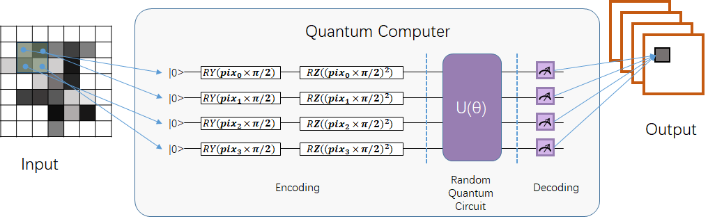
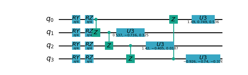
First we need encoding by inserting \(RY\) and \(RZ\) gates on each qubit, then, we constructed the parameter circuit through \(U3\) gate and \(Z\) gate . The sample is as follows:

class pyvqnet.qnn.qcnn.qconv.QConv(input_channels, output_channels, quantum_number, stride=(1, 1), padding=(0, 0), kernel_initializer=normal, machine: str = 'cpu', dtype=None, name='')¶

Quantum Convolution module. Replace Conv2D kernal with quantum circuits.Inputs to the conv module are of shape (batch_size, input_channels, height, width) reference Samuel et al. (2020).

Parameters:

input_channels – int - Number of input channels
output_channels – int - Number of kernels
quantum_number – int - Size of a single kernel.
stride – tuple - Stride, defaults to (1, 1)
padding – tuple - Padding, defaults to (0, 0)
kernel_initializer – callable - Defaults to normal
machine – str - cpu simulation.
dtype – The data type of the parameter, defaults: None, use the default data type kfloat32, which represents a 32-bit floating point number.
name – name of the output layer

Returns:

a quantum cnn class

Example:

from pyvqnet.tensor import tensor
from pyvqnet.qnn.qcnn.qconv import QConv
x = tensor.ones([1,3,4,4])
layer = QConv(input_channels=3, output_channels=2, quantum_number=4, stride=(2, 2))
y = layer(x)
print(y)

# [
# [[[-0.0889078, -0.0889078],
#  [-0.0889078, -0.0889078]],
# [[0.7992646, 0.7992646],
#  [0.7992646, 0.7992646]]]
# ]

QLinear¶

QLinear implements a quantum full connection algorithm. Firstly, the data is encoded into the quantum state, and then the final fully connected result is obtained through the derivation operation and measurement of the quantum circuit.

class pyvqnet.qnn.qlinear.QLinear(input_channels, output_channels, machine: str = 'cpu')¶

Quantum Linear module. Inputs to the linear module are of shape (input_channels, output_channels).This layer takes no variational quantum parameters.

Parameters:

input_channels – int - Number of input channels
output_channels – int - Number of output channels
machine – str - cpu simulation

Returns:

a quantum linear layer

Exmaple:

from pyvqnet.tensor import QTensor
from pyvqnet.qnn.qlinear import QLinear
params = [[0.37454012, 0.95071431, 0.73199394, 0.59865848, 0.15601864, 0.15599452],
[1.37454012, 0.95071431, 0.73199394, 0.59865848, 0.15601864, 0.15599452],
[1.37454012, 1.95071431, 0.73199394, 0.59865848, 0.15601864, 0.15599452],
[1.37454012, 1.95071431, 1.73199394, 1.59865848, 0.15601864, 0.15599452]]
m = QLinear(6, 2)
input = QTensor(params, requires_grad=True)
output = m(input)
output.backward()
print(output)

# [
#[0.0568473, 0.1264389],
#[0.1524036, 0.1264389],
#[0.1524036, 0.1442845],
#[0.1524036, 0.1442845]
# ]

grad¶

pyvqnet.qnn.quantumlayer.grad(quantum_prog_func, params *args)¶

The grad function provides an interface to compute the gradient of a user-designed subcircuit with parametric parameters. Users can use pyqpanda to design the line running function quantum_prog_func according to the following example, and send it as a parameter to the grad function. The second parameter of the grad function is the coordinates at which you want to calculate the gradient of the quantum logic gate parameters. The return value has shape [num of parameters,num of output].

Parameters:

quantum_prog_func – The quantum circuit operation function designed by pyqpanda.
params – The coordinates of the parameters whose gradient is to be obtained.
*args – additional arguments to the quantum_prog_func function.

Returns:

gradient of parameters

Examples:

from pyvqnet.qnn import grad, ProbsMeasure
import pyqpanda as pq

def pqctest(param):
    machine = pq.CPUQVM()
    machine.init_qvm()
    qubits = machine.qAlloc_many(2)
    circuit = pq.QCircuit()

    circuit.insert(pq.RX(qubits[0], param[0]))

    circuit.insert(pq.RY(qubits[1], param[1]))
    circuit.insert(pq.CNOT(qubits[0], qubits[1]))

    circuit.insert(pq.RX(qubits[1], param[2]))

    prog = pq.QProg()
    prog.insert(circuit)

    EXP = ProbsMeasure([1],prog,machine,qubits)
    return EXP


g = grad(pqctest, [0.1,0.2, 0.3])
print(g)
# [[-0.04673668  0.04673668]
# [-0.09442394  0.09442394]
# [-0.14409127  0.14409127]]

Quantum Gates¶

The way to deal with qubits is called quantum gates. Using quantum gates, we consciously evolve quantum states. Quantum gates are the basis of quantum algorithms.

Basic quantum gates¶

In VQNet, we use each logic gate of pyQPanda developed by the original quantum to build quantum circuit and conduct quantum simulation. The gates currently supported by pyQPanda can be defined in pyQPanda’s quantum gate section. In addition, VQNet also encapsulates some quantum gate combinations commonly used in quantum machine learning.

BasicEmbeddingCircuit¶

pyvqnet.qnn.template.BasicEmbeddingCircuit(input_feat, qlist)¶

Encodes n binary features into a basis state of n qubits.

For example, for features=([0, 1, 1]), the quantum system will be prepared in state \(|011 \rangle\).

Parameters:

input_feat – binary input of shape (n)
qlist – qlist that the template acts on

Returns:

quantum circuits

Example:

import numpy as np
import pyqpanda as pq
from pyvqnet.qnn.template import BasicEmbeddingCircuit
input_feat = np.array([1,1,0]).reshape([3])
m_machine = pq.init_quantum_machine(pq.QMachineType.CPU)

qlist = m_machine.qAlloc_many(3)
circuit = BasicEmbeddingCircuit(input_feat,qlist)
print(circuit)

#           ┌─┐
# q_0:  |0>─┤X├
#           ├─┤
# q_1:  |0>─┤X├
#           └─┘

AngleEmbeddingCircuit¶

pyvqnet.qnn.template.AngleEmbeddingCircuit(input_feat, qubits, rotation: str = 'X')¶

Encodes \(N\) features into the rotation angles of \(n\) qubits, where \(N \leq n\).

The rotations can be chosen as either : ‘X’ , ‘Y’ , ‘Z’, as defined by the rotation parameter:

rotation='X' uses the features as angles of RX rotations
rotation='Y' uses the features as angles of RY rotations
rotation='Z' uses the features as angles of RZ rotations

The length of features has to be smaller or equal to the number of qubits. If there are fewer entries in features than qlists, the circuit does not Applies the remaining rotation gates.

Parameters:

input_feat – numpy array which represents paramters
qubits – qubits allocated by pyQPanda
rotation – use what rotation ,default ‘X’

Returns:

quantum circuits

Example:

import numpy as np
import pyqpanda as pq
from pyvqnet.qnn.template import AngleEmbeddingCircuit
m_machine = pq.init_quantum_machine(pq.QMachineType.CPU)
m_qlist = m_machine.qAlloc_many(2)
m_clist = m_machine.cAlloc_many(2)
m_prog = pq.QProg()

input_feat = np.array([2.2, 1])
C = AngleEmbeddingCircuit(input_feat,m_qlist,'X')
print(C)
C = AngleEmbeddingCircuit(input_feat,m_qlist,'Y')
print(C)
C = AngleEmbeddingCircuit(input_feat,m_qlist,'Z')
print(C)
pq.destroy_quantum_machine(m_machine)

#           ┌────────────┐
# q_0:  |0>─┤RX(2.200000)├
#           ├────────────┤
# q_1:  |0>─┤RX(1.000000)├
#           └────────────┘



#           ┌────────────┐
# q_0:  |0>─┤RY(2.200000)├
#           ├────────────┤
# q_1:  |0>─┤RY(1.000000)├
#           └────────────┘



#           ┌────────────┐
# q_0:  |0>─┤RZ(2.200000)├
#           ├────────────┤
# q_1:  |0>─┤RZ(1.000000)├
#           └────────────┘

AmplitudeEmbeddingCircuit¶

pyvqnet.qnn.template.AmplitudeEmbeddingCircuit(input_feat, qubits)¶

Encodes \(2^n\) features into the amplitude vector of \(n\) qubits. To represent a valid quantum state vector, the L2-norm of features must be one.

Parameters:

input_feat – numpy array which represents paramters
qubits – qubits allocated by pyQPanda

Returns:

quantum circuits

Example:

import numpy as np
import pyqpanda as pq
from pyvqnet.qnn.template import AmplitudeEmbeddingCircuit
input_feat = np.array([2.2, 1, 4.5, 3.7])
m_machine = pq.init_quantum_machine(pq.QMachineType.CPU)
m_qlist = m_machine.qAlloc_many(2)
m_clist = m_machine.cAlloc_many(2)
m_prog = pq.QProg()
cir = AmplitudeEmbeddingCircuit(input_feat,m_qlist)
print(cir)
pq.destroy_quantum_machine(m_machine)

#                              ┌────────────┐     ┌────────────┐
# q_0:  |0>─────────────── ─── ┤RY(0.853255)├ ─── ┤RY(1.376290)├
#           ┌────────────┐ ┌─┐ └──────┬─────┘ ┌─┐ └──────┬─────┘
# q_1:  |0>─┤RY(2.355174)├ ┤X├ ───────■────── ┤X├ ───────■──────
#           └────────────┘ └─┘                └─┘

IQPEmbeddingCircuits¶

pyvqnet.qnn.template.IQPEmbeddingCircuits(input_feat, qubits, trep: int = 1)¶

Encodes \(n\) features into \(n\) qubits using diagonal gates of an IQP circuit.

The embedding was proposed by Havlicek et al. (2018).

The basic IQP circuit can be repeated by specifying n_repeats.

Parameters:

input_feat – numpy array which represents paramters
qubits – qubits allocated by pyQPanda
rep – repeat circuits block

Returns:

quantum circuits

Example:

import numpy as np
import pyqpanda as pq
from pyvqnet.qnn.template import IQPEmbeddingCircuits
m_machine = pq.init_quantum_machine(pq.QMachineType.CPU)
input_feat = np.arange(1,100)
qlist = m_machine.qAlloc_many(3)
circuit = IQPEmbeddingCircuits(input_feat,qlist,rep = 1)
print(circuit)

#           ┌─┐ ┌────────────┐
# q_0:  |0>─┤H├ ┤RZ(1.000000)├ ───■── ────────────── ───■── ───■── ────────────── ───■── ────── ────────────── ──────
#           ├─┤ ├────────────┤ ┌──┴─┐ ┌────────────┐ ┌──┴─┐    │                     │
# q_1:  |0>─┤H├ ┤RZ(2.000000)├ ┤CNOT├ ┤RZ(2.000000)├ ┤CNOT├ ───┼── ────────────── ───┼── ───■── ────────────── ───■──
#           ├─┤ ├────────────┤ └────┘ └────────────┘ └────┘ ┌──┴─┐ ┌────────────┐ ┌──┴─┐ ┌──┴─┐ ┌────────────┐ ┌──┴─┐
# q_2:  |0>─┤H├ ┤RZ(3.000000)├ ────── ────────────── ────── ┤CNOT├ ┤RZ(3.000000)├ ┤CNOT├ ┤CNOT├ ┤RZ(3.000000)├ ┤CNOT├
#           └─┘ └────────────┘                              └────┘ └────────────┘ └────┘ └────┘ └────────────┘ └────┘

RotCircuit¶

pyvqnet.qnn.template.RotCircuit(para, qubits)¶

Arbitrary single qubit rotation.Number of qlist should be 1,and number of parameters should be 3

\[\begin{split}R(\phi,\theta,\omega) = RZ(\omega)RY(\theta)RZ(\phi)= \begin{bmatrix} e^{-i(\phi+\omega)/2}\cos(\theta/2) & -e^{i(\phi-\omega)/2}\sin(\theta/2) \\ e^{-i(\phi-\omega)/2}\sin(\theta/2) & e^{i(\phi+\omega)/2}\cos(\theta/2) \end{bmatrix}.\end{split}\]

Parameters:

para – numpy array which represents paramters [phi, theta, omega]
qubits – qubits allocated by pyQPanda,only accepted single qubits.

Returns:

quantum circuits

Example:

import pyqpanda as pq
import numpy as np
from pyvqnet.tensor import QTensor
from pyvqnet.qnn.template import RotCircuit
import pyvqnet
m_machine = pq.init_quantum_machine(pq.QMachineType.CPU)
m_clist = m_machine.cAlloc_many(2)
m_prog = pq.QProg()
m_qlist = m_machine.qAlloc_many(1)
param = np.array([3,4,5])
c = pyvqnet.qnn.template.RotCircuit(param,m_qlist)
print(c)
pq.destroy_quantum_machine(m_machine)

#           ┌────────────┐ ┌────────────┐ ┌────────────┐
# q_0:  |0>─┤RZ(5.000000)├ ┤RY(4.000000)├ ┤RZ(3.000000)├
#           └────────────┘ └────────────┘ └────────────┘

CRotCircuit¶

pyvqnet.qnn.template.CRotCircuit(para, control_qubits, rot_qubits)¶

The controlled-Rot operator

\[\begin{split}CR(\phi, \theta, \omega) = \begin{bmatrix} 1 & 0 & 0 & 0 \\ 0 & 1 & 0 & 0\\ 0 & 0 & e^{-i(\phi+\omega)/2}\cos(\theta/2) & -e^{i(\phi-\omega)/2}\sin(\theta/2)\\ 0 & 0 & e^{-i(\phi-\omega)/2}\sin(\theta/2) & e^{i(\phi+\omega)/2}\cos(\theta/2) \end{bmatrix}.\end{split}\]

Parameters:

para – numpy array which represents paramters [phi, theta, omega]
control_qubits – control qubit allocated by pyQPanda
rot_qubits – Rot qubit allocated by pyQPanda

Returns:

quantum circuits

Example:

import numpy as np
import pyqpanda as pq
from pyvqnet.tensor import QTensor
from pyvqnet.qnn.template import CRotCircuit
m_machine = pq.init_quantum_machine(pq.QMachineType.CPU)
m_clist = m_machine.cAlloc_many(2)
m_prog = pq.QProg()
m_qlist = m_machine.qAlloc_many(1)
param = np.array([3,4,5])
control_qlist = m_machine.qAlloc_many(1)
c = CRotCircuit(QTensor(param),control_qlist,m_qlist)
print(c)
pq.destroy_quantum_machine(m_machine)

#           ┌────────────┐ ┌────────────┐ ┌────────────┐
# q_0:  |0>─┤RZ(5.000000)├ ┤RY(4.000000)├ ┤RZ(3.000000)├
#           └──────┬─────┘ └──────┬─────┘ └──────┬─────┘
# q_1:  |0>────────■────── ───────■────── ───────■──────

CSWAPcircuit¶

pyvqnet.qnn.template.CSWAPcircuit(qubits)¶

The controlled-swap circuit

\[\begin{split}CSWAP = \begin{bmatrix} 1 & 0 & 0 & 0 & 0 & 0 & 0 & 0 \\ 0 & 1 & 0 & 0 & 0 & 0 & 0 & 0 \\ 0 & 0 & 1 & 0 & 0 & 0 & 0 & 0 \\ 0 & 0 & 0 & 1 & 0 & 0 & 0 & 0 \\ 0 & 0 & 0 & 0 & 1 & 0 & 0 & 0 \\ 0 & 0 & 0 & 0 & 0 & 0 & 1 & 0 \\ 0 & 0 & 0 & 0 & 0 & 1 & 0 & 0 \\ 0 & 0 & 0 & 0 & 0 & 0 & 0 & 1 \end{bmatrix}.\end{split}\]

Note

The first qubits provided corresponds to the control qubit.

Parameters:: qubits – list of qubits allocated by pyQPanda the first qubits is control qubit. length of qlists have to be 3.
Returns:: quantum circuits

Example:

from pyvqnet.qnn.template import CSWAPcircuit
import pyqpanda as pq
m_machine = pq.init_quantum_machine(pq.QMachineType.CPU)

m_qlist = m_machine.qAlloc_many(3)

c = CSWAPcircuit([m_qlist[1],m_qlist[2],m_qlist[0]])
print(c)
pq.destroy_quantum_machine(m_machine)

# q_0:  |0>─X─
#           │
# q_1:  |0>─■─
#           │
# q_2:  |0>─X─

Controlled_Hadamard¶

pyvqnet.qnn.template.Controlled_Hadamard(qubits)¶

Controlled Hadamard logic gates.

\[\begin{split}CH = \begin{bmatrix} 1 & 0 & 0 & 0 \\ 0 & 1 & 0 & 0 \\ 0 & 0 & \frac{1}{\sqrt{2}} & \frac{1}{\sqrt{2}} \\ 0 & 0 & \frac{1}{\sqrt{2}} & -\frac{1}{\sqrt{2}} \end{bmatrix}.\end{split}\]

Parameters:: qubits – Qubits requested using pyqpanda.

Examples:

import pyqpanda as pq

machine = pq.CPUQVM()
machine.init_qvm()
qubits = machine.qAlloc_many(2)
from pyvqnet.qnn import Controlled_Hadamard

cir = Controlled_Hadamard(qubits)
print(cir)
# q_0:  |0>──────────────── ──■─ ──────────────
#           ┌─────────────┐ ┌─┴┐ ┌────────────┐
# q_1:  |0>─┤RY(-0.785398)├ ┤CZ├ ┤RY(0.785398)├
#           └─────────────┘ └──┘ └────────────┘

CCZ¶

pyvqnet.qnn.template.CCZ(qubits)¶

Controlled-controlled-Z (controlled-controlled-Z) logic gate.

\[\begin{split}CCZ = \begin{pmatrix} 1 & 0 & 0 & 0 & 0 & 0 & 0 & 0\\ 0 & 1 & 0 & 0 & 0 & 0 & 0 & 0\\ 0 & 0 & 1 & 0 & 0 & 0 & 0 & 0\\ 0 & 0 & 0 & 1 & 0 & 0 & 0 & 0\\ 0 & 0 & 0 & 0 & 1 & 0 & 0 & 0\\ 0 & 0 & 0 & 0 & 0 & 1 & 0 & 0\\ 0 & 0 & 0 & 0 & 0 & 0 & 1 & 0\\ 0 & 0 & 0 & 0 & 0 & 0 & 0 & -1 \end{pmatrix}\end{split}\]

Parameters:: qubits – Qubits requested using pyqpanda.
Returns:: pyqpanda QCircuit

Example:

import pyqpanda as pq

machine = pq.CPUQVM()
machine.init_qvm()
qubits = machine.qAlloc_many(3)
from pyvqnet.qnn import CCZ

cir = CCZ(qubits)
print(cir)
# q_0:  |0>─────── ─────── ───■── ─── ────── ─────── ───■── ───■── ┤T├──── ───■──
#                             │              ┌─┐        │   ┌──┴─┐ ├─┴───┐ ┌──┴─┐
# q_1:  |0>────■── ─────── ───┼── ─── ───■── ┤T├──── ───┼── ┤CNOT├ ┤T.dag├ ┤CNOT├
#           ┌──┴─┐ ┌─────┐ ┌──┴─┐ ┌─┐ ┌──┴─┐ ├─┴───┐ ┌──┴─┐ ├─┬──┘ ├─┬───┘ ├─┬──┘
# q_2:  |0>─┤CNOT├ ┤T.dag├ ┤CNOT├ ┤T├ ┤CNOT├ ┤T.dag├ ┤CNOT├ ┤T├─── ┤H├──── ┤H├───
#           └────┘ └─────┘ └────┘ └─┘ └────┘ └─────┘ └────┘ └─┘    └─┘     └─┘

BlockEncode¶

pyvqnet.qnn.template.BlockEncode(A, qlists)¶

Construct a single pyqpanda circuit \(U(A)\) such that an arbitrary matrix \(A\) is encoded in the top left block.

Parameters:

A – The input matrix encoded in the circuit.
qlists – List of qubits to encode.

Returns:

A pyqpanda QCircuit.

Example:

from pyvqnet.tensor import QTensor
import pyvqnet
import pyqpanda as pq
from pyvqnet.qnn import BlockEncode
A = QTensor([[0.1, 0.2], [0.3, 0.4]], dtype=pyvqnet.kfloat32)
machine = pq.CPUQVM()
machine.init_qvm()
qlist = machine.qAlloc_many(2)
cbits = machine.cAlloc_many(2)

cir = BlockEncode(A, qlist)

prog = pq.QProg()
prog.insert(cir)
result = machine.directly_run(prog)
print(cir)

#           ┌───────────┐
# q_0:  |0>─┤0          ├
#           │  Unitary  │
# q_1:  |0>─┤1          ├
#           └───────────┘

Random_Init_Quantum_State¶

pyvqnet.qnn.template.Random_Init_Quantum_State(qlists)¶

Use amplitude encoding to generate arbitrary quantum initial states and encode them onto the wire. Note that the depth of the line can vary greatly due to amplitude encoding.

Parameters:: qlists – Qubits requested by pyqpanda.
Returns:: pyqpanda QCircuit.

Example:

import pyqpanda as pq
from pyvqnet.qnn.template import Random_Init_Quantum_State
cir = pq. QCircuit()

m_machine = pq.init_quantum_machine(pq.QMachineType.CPU)

m_qlist = m_machine.qAlloc_many(3)
c = Random_Init_Quantum_State(m_qlist)
print(c)

import pyqpanda as pq
from pyvqnet.qnn.template import Random_Init_Quantum_State
cir = pq.QCircuit()

m_machine = pq.init_quantum_machine(pq.QMachineType.CPU)

m_qlist = m_machine.qAlloc_many(3)
c = Random_Init_Quantum_State(m_qlist)
print(c)

# q_0:  |0>─────────────── ─── ────────────── ─── ┤RY(0.583047)├ ─── ┤RY(0.176308)├ ─── ────────────── >
#                              ┌────────────┐ ┌─┐ └──────┬─────┘ ┌─┐ └──────┬─────┘     ┌────────────┐ >
# q_1:  |0>─────────────── ─── ┤RY(1.062034)├ ┤X├ ───────■────── ┤X├ ───────■────── ─── ┤RY(1.724022)├ >
#           ┌────────────┐ ┌─┐ └──────┬─────┘ └┬┘        │       └┬┘        │       ┌─┐ └──────┬─────┘ >
# q_2:  |0>─┤RY(1.951150)├ ┤X├ ───────■────── ─■─ ───────■────── ─■─ ───────■────── ┤X├ ───────■────── >
#           └────────────┘ └─┘                                                      └─┘                >

#              ┌────────────┐     ┌────────────┐
# q_0:  |0>─── ┤RY(1.251911)├ ─── ┤RY(1.389063)├
#          ┌─┐ └──────┬─────┘ ┌─┐ └──────┬─────┘
# q_1:  |0>┤X├ ───────■────── ┤X├ ───────■──────
#          └┬┘        │       └┬┘        │
# q_2:  |0>─■─ ───────■────── ─■─ ───────■──────

FermionicSingleExcitation¶

pyvqnet.qnn.template.FermionicSingleExcitation(weight, wires, qubits)¶

A coupled cluster single-excitation operator for exponentiating the tensor product of a Pauli matrix. The matrix form is given by:

\[\hat{U}_{pr}(\theta) = \mathrm{exp} \{ \theta_{pr} (\hat{c}_p^\dagger \hat{c}_r -\mathrm{H.c.}) \}\]

Parameters:

weight – Variable parameter on qubit p.
wires – Indicates a subset of qubit indices in the interval [r, p]. Minimum length must be 2. The first index value is interpreted as r and the last index value as p. The intermediate index is acted on by the CNOT gate to calculate the parity of the qubit set.
qubits – Qubits applied by pyqpanda.

Examples:

from pyvqnet.qnn import FermionicSingleExcitation, expval

weight = 0.5
import pyqpanda as pq
machine = pq.CPUQVM()
machine.init_qvm()
qlists = machine.qAlloc_many(3)

cir = FermionicSingleExcitation(weight, [1, 0, 2], qlists)

prog = pq.QProg()
prog.insert(cir)
pauli_dict = {'Z0': 1}
exp2 = expval(machine, prog, pauli_dict, qlists)
print(f"vqnet {exp2}")
#vqnet 1000000013

FermionicDoubleExcitation¶

pyvqnet.qnn.template.FermionicDoubleExcitation(weight, wires1, wires2, qubits)¶

The coupled clustering dual excitation operator that exponentiates the tensor product of the Pauli matrix, the matrix form is given by:

\[\hat{U}_{pqrs}(\theta) = \mathrm{exp} \{ \theta (\hat{c}_p^\dagger \hat{c}_q^\dagger \hat{c}_r \hat{c}_s - \mathrm{H.c.}) \}\]

where \(\hat{c}\) and \(\hat{c}^\dagger\) are the fermion annihilation and Create operators and indices \(r, s\) and \(p, q\) in the occupied and are empty molecular orbitals, respectively. Use the Jordan-Wigner transformation The fermion operator defined above can be written as According to the Pauli matrix (for more details, see arXiv:1805.04340)

\[\begin{split}\hat{U}_{pqrs}(\theta) = \mathrm{exp} \Big\{ \frac{i\theta}{8} \bigotimes_{b=s+1}^{r-1} \hat{Z}_b \bigotimes_{a=q+1}^{p-1} \hat{Z}_a (\hat{X}_s \hat{X}_r \hat{Y}_q \hat{X}_p + \hat{Y}_s \hat{X}_r \hat{Y}_q \hat{Y}_p +\\ \hat{X}_s \hat{Y}_r \hat{Y}_q \hat{Y}_p + \hat{X}_s \hat{X}_r \hat{X}_q \hat{Y}_p - \mathrm{H.c.} ) \Big\}\end{split}\]

Parameters:

weight – variable parameter
wires1 – The index list of the represented qubits occupies a subset of qubits in the interval [s, r]. The first index is interpreted as s, the last as r. CNOT gates operate on intermediate indices to compute the parity of a set of qubits.
wires2 – The index list of the represented qubits occupies a subset of qubits in the interval [q, p]. The first index is interpreted as q, the last as p. CNOT gates operate on intermediate indices to compute the parity of a set of qubits.
qubits – Qubits applied by pyqpanda.

Returns:

pyqpanda QCircuit

Examples:

import pyqpanda as pq
from pyvqnet.qnn import FermionicDoubleExcitation, expval
machine = pq.CPUQVM()
machine.init_qvm()
qlists = machine.qAlloc_many(5)
weight = 1.5
cir = FermionicDoubleExcitation(weight,
                                wires1=[0, 1],
                                wires2=[2, 3, 4],
                                qubits=qlists)

prog = pq.QProg()
prog.insert(cir)
pauli_dict = {'Z0': 1}
exp2 = expval(machine, prog, pauli_dict, qlists)
print(f"vqnet {exp2}")
#vqnet 1000000058

UCCSD¶

pyvqnet.qnn.template.UCCSD(weights, wires, s_wires, d_wires, init_state, qubits)¶

Realize the unitary coupled cluster single-excitation and double-excitation design (UCCSD). UCCSD is the proposed VQE design, commonly used to run quantum chemistry simulations.

Within the first-order Trotter approximation, the UCCSD unitary function is given by:

\[\hat{U}(\vec{\theta}) = \prod_{p > r} \mathrm{exp} \Big\{\theta_{pr} (\hat{c}_p^\dagger \hat{c}_r-\mathrm{H.c.}) \Big\} \prod_{p > q > r > s} \mathrm{exp} \Big\{\theta_{pqrs} (\hat{c}_p^\dagger \hat{c}_q^\dagger \hat{c}_r \hat{c}_s-\mathrm{H.c.}) \Big\}\]

where \(\hat{c}\) and \(\hat{c}^\dagger\) are the fermion annihilation and Create operators and indices \(r, s\) and \(p, q\) in the occupied and are empty molecular orbitals, respectively. (For more details see arXiv:1805.04340):

Parameters:

weights – (len(s_wires)+ len(d_wires)) tensor containing the size of the parameters \(\theta_{pr}\) and \(\theta_{pqrs}\) input Z rotation FermionicSingleExcitation and FermionicDoubleExcitation.
wires – qubit index for template action
s_wires – sequence of lists containing qubit indices [r,...,p] produced by a single excitation \(\vert r, p \rangle = \hat{c}_p^\dagger \hat{c}_r \vert \mathrm{HF} \rangle\), where \(\vert \mathrm{HF} \rangle\) denotes the Hartee-Fock reference state.
d_wires – list sequence, each list contains two lists specify indices [s, ...,r] and [q,...,p] Define double excitation \(\vert s, r, q, p \rangle = \hat{c}_p^\dagger \hat{c}_q^\dagger \hat{c}_r\hat{c}_s \ vert \mathrm{HF} \rangle\).
init_state – length len(wires) occupation-number vector representation high frequency state. init_state is the qubit initialization state.
qubits – Qubits allocated by pyqpanda.

Examples:

import pyqpanda as pq
from pyvqnet.tensor import tensor
from pyvqnet.qnn import UCCSD, expval
machine = pq.CPUQVM()
machine.init_qvm()
qlists = machine.qAlloc_many(6)
weight = tensor.zeros([8])
cir = UCCSD(weight,wires = [0,1,2,3,4,5,6],
                                s_wires=[[0, 1, 2], [0, 1, 2, 3, 4], [1, 2, 3], [1, 2, 3, 4, 5]],
                                d_wires=[[[0, 1], [2, 3]], [[0, 1], [2, 3, 4, 5]], [[0, 1], [3, 4]], [[0, 1], [4, 5]]],
                                init_state=[1, 1, 0, 0, 0, 0],
                                qubits=qlists)

prog = pq.QProg()
prog.insert(cir)
pauli_dict = {'Z0': 1}
exp2 = expval(machine, prog, pauli_dict, qlists)
print(f"vqnet {exp2}")
#vqnet -1000000004

QuantumPoolingCircuit¶

pyvqnet.qnn.template.QuantumPoolingCircuit(sources_wires, sinks_wires, params, qubits)¶

A quantum circuit that downsamples data. To reduce the number of qubits in our circuit, we first create pairs of qubits in our system. After initially pairing all qubits, we apply our generalized 2-qubit unitary to each pair. After applying the two-qubit unitary, we ignore one qubit in each pair of qubits for the rest of the neural network.

Parameters:

sources_wires – Source qubit indices that will be ignored.
sinks_wires – Destination qubit indices that will be kept.
params – Input parameters.
qubits – list of qubits allocated by pyqpanda.

Returns:

pyqpanda QCircuit

Examples:

from pyvqnet.qnn import QuantumPoolingCircuit
import pyqpanda as pq
from pyvqnet import tensor
machine = pq.CPUQVM()
machine.init_qvm()
qlists = machine.qAlloc_many(4)
p = tensor.full([6], 0.35)
cir = QuantumPoolingCircuit([0, 1], [2, 3], p, qlists)
print(cir)

#                           ┌────┐ ┌────────────┐                           !
# >
# q_0:  |0>──────────────── ┤CNOT├ ┤RZ(0.350000)├ ───■── ────────────── ────! ─────────────── ────── ──────────────
# >
#                           └──┬─┘ └────────────┘    │                      !                 ┌────┐ ┌────────────┐
# >
# q_1:  |0>──────────────── ───┼── ────────────── ───┼── ────────────── ────! ─────────────── ┤CNOT├ ┤RZ(0.350000)├
# >
#           ┌─────────────┐    │   ┌────────────┐ ┌──┴─┐ ┌────────────┐     !                 └──┬─┘ └────────────┘
# >
# q_2:  |0>─┤RZ(-1.570796)├ ───■── ┤RY(0.350000)├ ┤CNOT├ ┤RY(0.350000)├ ────! ─────────────── ───┼── ──────────────
# >
#           └─────────────┘        └────────────┘ └────┘ └────────────┘     ! ┌─────────────┐    │   ┌────────────┐
# >
# q_3:  |0>──────────────── ────── ────────────── ────── ────────────── ────! ┤RZ(-1.570796)├ ───■── ┤RY(0.350000)├
# >
#                                                                           ! └─────────────┘        └────────────┘
# >
#                                    !
# q_0:  |0>────── ────────────── ────!
#                                    !
# q_1:  |0>───■── ────────────── ────!
#             │                      !
# q_2:  |0>───┼── ────────────── ────!
#          ┌──┴─┐ ┌────────────┐     !
# q_3:  |0>┤CNOT├ ┤RY(0.350000)├ ────!

Commonly used quantum circuits¶

VQNet provides some quantum circuits commonly used in quantum machine learning research.

HardwareEfficientAnsatz¶

class pyvqnet.qnn.ansatz.HardwareEfficientAnsatz(n_qubits, single_rot_gate_list, qubits, entangle_gate='CNOT', entangle_rules='linear', depth=1)¶

The implementation of Hardware Efficient Ansatz introduced in the paper: Hardware-efficient Variational Quantum Eigensolver for Small Molecules.

Parameters:

n_qubits – Number of qubits.
single_rot_gate_list – A single qubit rotation gate list is constructed by one or several rotation gate that act on every qubit.Currently support Rx, Ry, Rz.
qubits – Qubits allocated by pyqpanda api.
entangle_gate – The non parameterized entanglement gate.CNOT,CZ is supported.default:CNOT.
entangle_rules – How entanglement gate is used in the circuit. linear means the entanglement gate will be act on every neighboring qubits. all means the entanglment gate will be act on any two qbuits. Default: linear.
depth – The depth of ansatz, default:1.

Example:

import pyqpanda as pq
from pyvqnet.tensor import QTensor,tensor
from pyvqnet.qnn import HardwareEfficientAnsatz
machine = pq.CPUQVM()
machine.init_qvm()
qlist = machine.qAlloc_many(4)
c = HardwareEfficientAnsatz(4, ["rx", "RY", "rz"],
                            qlist,
                            entangle_gate="cnot",
                            entangle_rules="linear",
                            depth=1)
w = tensor.ones([c.get_para_num()])

cir = c.create_ansatz(w)
print(cir)
#           ┌────────────┐ ┌────────────┐ ┌────────────┐        ┌────────────┐ ┌────────────┐ ┌────────────┐
# q_0:  |0>─┤RX(1.000000)├ ┤RY(1.000000)├ ┤RZ(1.000000)├ ───■── ┤RX(1.000000)├ ┤RY(1.000000)├ ┤RZ(1.000000)├ ────────────── ──────────────
#           ├────────────┤ ├────────────┤ ├────────────┤ ┌──┴─┐ └────────────┘ ├────────────┤ ├────────────┤ ┌────────────┐
# q_1:  |0>─┤RX(1.000000)├ ┤RY(1.000000)├ ┤RZ(1.000000)├ ┤CNOT├ ───■────────── ┤RX(1.000000)├ ┤RY(1.000000)├ ┤RZ(1.000000)├ ──────────────
#           ├────────────┤ ├────────────┤ ├────────────┤ └────┘ ┌──┴─┐         └────────────┘ ├────────────┤ ├────────────┤ ┌────────────┐
# q_2:  |0>─┤RX(1.000000)├ ┤RY(1.000000)├ ┤RZ(1.000000)├ ────── ┤CNOT├──────── ───■────────── ┤RX(1.000000)├ ┤RY(1.000000)├ ┤RZ(1.000000)├
#           ├────────────┤ ├────────────┤ ├────────────┤        └────┘         ┌──┴─┐         ├────────────┤ ├────────────┤ ├────────────┤
# q_3:  |0>─┤RX(1.000000)├ ┤RY(1.000000)├ ┤RZ(1.000000)├ ────── ────────────── ┤CNOT├──────── ┤RX(1.000000)├ ┤RY(1.000000)├ ┤RZ(1.000000)├
#           └────────────┘ └────────────┘ └────────────┘                       └────┘         └────────────┘ └────────────┘ └────────────┘

BasicEntanglerTemplate¶

class pyvqnet.qnn.template.BasicEntanglerTemplate(weights=None, num_qubits=1, rotation=pyqpanda.RX)¶

Layers consisting of one-parameter single-qubit rotations on each qubit, followed by a closed chain or ring of CNOT gates.

The ring of CNOT gates connects every qubit with its neighbour, with the last qubit being considered as a neighbour to the first qubit.

The number of layers \(L\) is determined by the first dimension of the argument weights.

Parameters:

weights – Weight tensor of shape (L, len(qubits)) . Each weight is used as a parameter for the rotation, default: None, use random tensor with shape (1,1) .
num_qubits – number of qubits, default: 1.
rotation – one-parameter single-qubit gate to use, default: pyqpanda.RX

Example:

import pyqpanda as pq
import numpy as np
from pyvqnet.qnn.template import BasicEntanglerTemplate
np.random.seed(42)
num_qubits = 5
shape = [1, num_qubits]
weights = np.random.random(size=shape)

machine = pq.CPUQVM()
machine.init_qvm()
qubits = machine.qAlloc_many(num_qubits)

circuit = BasicEntanglerTemplate(weights=weights, num_qubits=num_qubits, rotation=pq.RZ)
result = circuit.create_circuit(qubits)
circuit.print_circuit(qubits)

prob = machine.prob_run_dict(result, qubits[0], -1)
prob = list(prob.values())
print(prob)
#           ┌────────────┐                             ┌────┐
# q_0:  |0>─┤RZ(0.374540)├ ───■── ────── ────── ────── ┤CNOT├
#           ├────────────┤ ┌──┴─┐                      └──┬─┘
# q_1:  |0>─┤RZ(0.950714)├ ┤CNOT├ ───■── ────── ────── ───┼──
#           ├────────────┤ └────┘ ┌──┴─┐                  │
# q_2:  |0>─┤RZ(0.731994)├ ────── ┤CNOT├ ───■── ────── ───┼──
#           ├────────────┤        └────┘ ┌──┴─┐           │
# q_3:  |0>─┤RZ(0.598658)├ ────── ────── ┤CNOT├ ───■── ───┼──
#           ├────────────┤               └────┘ ┌──┴─┐    │
# q_4:  |0>─┤RZ(0.156019)├ ────── ────── ────── ┤CNOT├ ───■──
#           └────────────┘                      └────┘

# [1.0, 0.0]

StronglyEntanglingTemplate¶

class pyvqnet.qnn.template.StronglyEntanglingTemplate(weights=None, num_qubits=1, ranges=None)¶

Layers consisting of single qubit rotations and entanglers, inspired by the circuit-centric classifier design .

The argument weights contains the weights for each layer. The number of layers \(L\) is therefore derived from the first dimension of weights.

The 2-qubit CNOT gate, act on the \(M\) number of qubits, \(i = 1,...,M\). The second qubit of each gate is given by \((i+r)\mod M\), where \(r\) is a hyperparameter called the range, and \(0 < r < M\).

Parameters:

weights – weight tensor of shape (L, M, 3) , default: None, use random tensor with shape (1,1,3) .
num_qubits – number of qubits, default: 1.
ranges – sequence determining the range hyperparameter for each subsequent layer; default: None, using \(r=l \mod M\) for the \(l\) th layer and \(M\) qubits.

Example:

import pyqpanda as pq
import numpy as np
from pyvqnet.qnn.template import StronglyEntanglingTemplate
np.random.seed(42)
num_qubits = 3
shape = [2, num_qubits, 3]
weights = np.random.random(size=shape)

machine = pq.CPUQVM()  # outside
machine.init_qvm()  # outside
qubits = machine.qAlloc_many(num_qubits)

circuit = StronglyEntanglingTemplate(weights, num_qubits=num_qubits)
result = circuit.create_circuit(qubits)
circuit.print_circuit(qubits)

prob = machine.prob_run_dict(result, qubits[0], -1)
prob = list(prob.values())
print(prob)
#           ┌────────────┐ ┌────────────┐ ┌────────────┐               ┌────┐             ┌────────────┐ >
# q_0:  |0>─┤RZ(0.374540)├ ┤RY(0.950714)├ ┤RZ(0.731994)├ ───■── ────── ┤CNOT├──────────── ┤RZ(0.708073)├ >
#           ├────────────┤ ├────────────┤ ├────────────┤ ┌──┴─┐        └──┬┬┴───────────┐ ├────────────┤ >
# q_1:  |0>─┤RZ(0.598658)├ ┤RY(0.156019)├ ┤RZ(0.155995)├ ┤CNOT├ ───■── ───┼┤RZ(0.832443)├ ┤RY(0.212339)├ >
#           ├────────────┤ ├────────────┤ ├────────────┤ └────┘ ┌──┴─┐    │└────────────┘ ├────────────┤ >
# q_2:  |0>─┤RZ(0.058084)├ ┤RY(0.866176)├ ┤RZ(0.601115)├ ────── ┤CNOT├ ───■────────────── ┤RZ(0.183405)├ >
#           └────────────┘ └────────────┘ └────────────┘        └────┘                    └────────────┘ >
#
#          ┌────────────┐ ┌────────────┐        ┌────┐
# q_0:  |0>┤RY(0.020584)├ ┤RZ(0.969910)├ ───■── ┤CNOT├ ──────
#          ├────────────┤ └────────────┘    │   └──┬─┘ ┌────┐
# q_1:  |0>┤RZ(0.181825)├ ────────────── ───┼── ───■── ┤CNOT├
#          ├────────────┤ ┌────────────┐ ┌──┴─┐        └──┬─┘
# q_2:  |0>┤RY(0.304242)├ ┤RZ(0.524756)├ ┤CNOT├ ────── ───■──
#          └────────────┘ └────────────┘ └────┘
#[0.6881335561525671, 0.31186644384743273]

ComplexEntangelingTemplate¶

class pyvqnet.qnn.ComplexEntangelingTemplate(weights, num_qubits, depth)¶

A strongly entangled layer consisting of U3 gates and CNOT gates. This circuit template is from the following paper: https://arxiv.org/abs/1804.00633.

Parameters:

weights – parameter, shape of [depth,num_qubits,3]
num_qubits – Number of qubits.
depth – The depth of the subcircuit.

Example:

from pyvqnet.qnn import ComplexEntangelingTemplate
import pyqpanda as pq
from pyvqnet. tensor import *
depth=3
num_qubits = 8
shape = [depth, num_qubits, 3]
weights = tensor.randn(shape)

machine = pq.CPUQVM()
machine.init_qvm()
qubits = machine.qAlloc_many(num_qubits)

circuit = ComplexEntangelingTemplate(weights, num_qubits=num_qubits,depth=depth)
result = circuit. create_circuit(qubits)
circuit. print_circuit(qubits)


# q_0:  |0>─┤U3(1.115555,-0.025096,1.326895)├── ───■── ────── ───────────────────────────────── ────────────────────────────────── >
#           ├───────────────────────────────┴─┐ ┌──┴─┐        ┌───────────────────────────────┐                                    >
# q_1:  |0>─┤U3(-0.884622,-0.239700,-0.701955)├ ┤CNOT├ ───■── ┤U3(0.811768,0.537290,-0.433107)├ ────────────────────────────────── >
#           ├────────────────────────────────┬┘ └────┘ ┌──┴─┐ └───────────────────────────────┘ ┌────────────────────────────────┐ >
# q_2:  |0>─┤U3(-0.387148,-0.322480,0.238582)├─ ────── ┤CNOT├ ───■───────────────────────────── ┤U3(-0.188015,-1.828407,0.070222)├ >
#           ├────────────────────────────────┤         └────┘ ┌──┴─┐                            └────────────────────────────────┘ >
# q_3:  |0>─┤U3(-0.679633,1.638090,-1.341497)├─ ────── ────── ┤CNOT├─────────────────────────── ───■────────────────────────────── >
#           ├──────────────────────────────┬─┘                └────┘                            ┌──┴─┐                             >
# q_4:  |0>─┤U3(2.073888,1.251795,0.238305)├─── ────── ────── ───────────────────────────────── ┤CNOT├──────────────────────────── >
#           ├──────────────────────────────┤                                                    └────┘                             >
# q_5:  |0>─┤U3(0.247473,2.772012,1.864166)├─── ────── ────── ───────────────────────────────── ────────────────────────────────── >
#           ├──────────────────────────────┴─┐                                                                                     >
# q_6:  |0>─┤U3(-1.421337,-0.866551,0.739282)├─ ────── ────── ───────────────────────────────── ────────────────────────────────── >
#           ├────────────────────────────────┤                                                                                     >
# q_7:  |0>─┤U3(-3.707045,0.690364,-0.979904)├─ ────── ────── ───────────────────────────────── ────────────────────────────────── >
#           └────────────────────────────────┘                                                                                     >

#                                                                                                                 >
# q_0:  |0>────────────────────────────────── ────────────────────────────────── ──────────────────────────────── >
#                                                                                                                 >
# q_1:  |0>────────────────────────────────── ────────────────────────────────── ──────────────────────────────── >
#                                                                                                                 >
# q_2:  |0>────────────────────────────────── ────────────────────────────────── ──────────────────────────────── >
#          ┌────────────────────────────────┐                                                                     >
# q_3:  |0>┤U3(0.516395,-0.823623,-0.804430)├ ────────────────────────────────── ──────────────────────────────── >
#          └────────────────────────────────┘ ┌────────────────────────────────┐                                  >
# q_4:  |0>───■────────────────────────────── ┤U3(-1.420068,1.063462,-0.107385)├ ──────────────────────────────── >
#          ┌──┴─┐                             └────────────────────────────────┘ ┌──────────────────────────────┐ >
# q_5:  |0>┤CNOT├──────────────────────────── ───■────────────────────────────── ┤U3(0.377809,0.204278,0.386830)├ >
#          └────┘                             ┌──┴─┐                             └──────────────────────────────┘ >
# q_6:  |0>────────────────────────────────── ┤CNOT├──────────────────────────── ───■──────────────────────────── >
#                                             └────┘                             ┌──┴─┐                           >
# q_7:  |0>────────────────────────────────── ────────────────────────────────── ┤CNOT├────────────────────────── >
#                                                                                └────┘                           >

#          ┌────┐                                 ┌────────────────────────────────┐                                                  >
# q_0:  |0>┤CNOT├──────────────────────────────── ┤U3(-0.460444,-1.150054,0.318044)├ ───■── ────── ────────────────────────────────── >
#          └──┬─┘                                 └────────────────────────────────┘ ┌──┴─┐        ┌────────────────────────────────┐ >
# q_1:  |0>───┼────────────────────────────────── ────────────────────────────────── ┤CNOT├ ───■── ┤U3(-1.255487,0.589956,-0.378491)├ >
#             │                                                                      └────┘ ┌──┴─┐ └────────────────────────────────┘ >
# q_2:  |0>───┼────────────────────────────────── ────────────────────────────────── ────── ┤CNOT├ ───■────────────────────────────── >
#             │                                                                             └────┘ ┌──┴─┐                             >
# q_3:  |0>───┼────────────────────────────────── ────────────────────────────────── ────── ────── ┤CNOT├──────────────────────────── >
#             │                                                                                    └────┘                             >
# q_4:  |0>───┼────────────────────────────────── ────────────────────────────────── ────── ────── ────────────────────────────────── >
#             │                                                                                                                       >
# q_5:  |0>───┼────────────────────────────────── ────────────────────────────────── ────── ────── ────────────────────────────────── >
#             │┌────────────────────────────────┐                                                                                     >
# q_6:  |0>───┼┤U3(-0.760777,-0.867848,0.016680)├ ────────────────────────────────── ────── ────── ────────────────────────────────── >
#             │└────────────────────────────────┘ ┌────────────────────────────────┐                                                  >
# q_7:  |0>───■────────────────────────────────── ┤U3(-1.462434,-0.173843,1.211081)├ ────── ────── ────────────────────────────────── >
#                                                 └────────────────────────────────┘                                                  >

#                                                                                                               >
# q_0:  |0>───────────────────────────────── ───────────────────────────────── ──────────────────────────────── >
#                                                                                                               >
# q_1:  |0>───────────────────────────────── ───────────────────────────────── ──────────────────────────────── >
#          ┌───────────────────────────────┐                                                                    >
# q_2:  |0>┤U3(0.558638,0.218889,-0.241834)├ ───────────────────────────────── ──────────────────────────────── >
#          └───────────────────────────────┘ ┌───────────────────────────────┐                                  >
# q_3:  |0>───■───────────────────────────── ┤U3(0.740361,-0.336978,0.171089)├ ──────────────────────────────── >
#          ┌──┴─┐                            └───────────────────────────────┘ ┌──────────────────────────────┐ >
# q_4:  |0>┤CNOT├─────────────────────────── ───■───────────────────────────── ┤U3(0.585393,0.204842,0.682543)├ >
#          └────┘                            ┌──┴─┐                            └──────────────────────────────┘ >
# q_5:  |0>───────────────────────────────── ┤CNOT├─────────────────────────── ───■──────────────────────────── >
#                                            └────┘                            ┌──┴─┐                           >
# q_6:  |0>───────────────────────────────── ───────────────────────────────── ┤CNOT├────────────────────────── >
#                                                                              └────┘                           >
# q_7:  |0>───────────────────────────────── ───────────────────────────────── ──────────────────────────────── >
#                                                                                                               >

#                                              ┌────┐                               ┌───────────────────────────────┐ >
# q_0:  |0>─────────────────────────────────── ┤CNOT├────────────────────────────── ┤U3(0.657827,1.434924,-0.328996)├ >
#                                              └──┬─┘                               └───────────────────────────────┘ >
# q_1:  |0>─────────────────────────────────── ───┼──────────────────────────────── ───────────────────────────────── >
#                                                 │                                                                   >
# q_2:  |0>─────────────────────────────────── ───┼──────────────────────────────── ───────────────────────────────── >
#                                                 │                                                                   >
# q_3:  |0>─────────────────────────────────── ───┼──────────────────────────────── ───────────────────────────────── >
#                                                 │                                                                   >
# q_4:  |0>─────────────────────────────────── ───┼──────────────────────────────── ───────────────────────────────── >
#          ┌─────────────────────────────────┐    │                                                                   >
# q_5:  |0>┤U3(-2.134247,-0.783461,-0.200094)├ ───┼──────────────────────────────── ───────────────────────────────── >
#          └─────────────────────────────────┘    │┌──────────────────────────────┐                                   >
# q_6:  |0>───■─────────────────────────────── ───┼┤U3(1.816030,0.572931,1.683584)├ ───────────────────────────────── >
#          ┌──┴─┐                                 │└──────────────────────────────┘ ┌───────────────────────────────┐ >
# q_7:  |0>┤CNOT├───────────────────────────── ───■──────────────────────────────── ┤U3(0.661537,0.214565,-0.325014)├ >
#          └────┘                                                                   └───────────────────────────────┘ >

#                                                           ┌────┐
# q_0:  |0>───■── ────── ────── ────── ────── ────── ────── ┤CNOT├
#          ┌──┴─┐                                           └──┬─┘
# q_1:  |0>┤CNOT├ ───■── ────── ────── ────── ────── ────── ───┼──
#          └────┘ ┌──┴─┐                                       │
# q_2:  |0>────── ┤CNOT├ ───■── ────── ────── ────── ────── ───┼──
#                 └────┘ ┌──┴─┐                                │
# q_3:  |0>────── ────── ┤CNOT├ ───■── ────── ────── ────── ───┼──
#                        └────┘ ┌──┴─┐                         │
# q_4:  |0>────── ────── ────── ┤CNOT├ ───■── ────── ────── ───┼──
#                               └────┘ ┌──┴─┐                  │
# q_5:  |0>────── ────── ────── ────── ┤CNOT├ ───■── ────── ───┼──
#                                      └────┘ ┌──┴─┐           │
# q_6:  |0>────── ────── ────── ────── ────── ┤CNOT├ ───■── ───┼──
#                                             └────┘ ┌──┴─┐    │
# q_7:  |0>────── ────── ────── ────── ────── ────── ┤CNOT├ ───■──

Quantum_Embedding¶

class pyvqnet.qnn.Quantum_Embedding(qubits, machine, num_repetitions_input, depth_input, num_unitary_layers, num_repetitions)¶

Use RZ,RY,RZ to create variational quantum circuits that encode classical data into quantum states. See Quantum embeddings for machine learning. After the class is initialized, its member function compute_circuit is a running function, which can be input as a parameter. The QuantumLayerV2 class can utilize compute_circuit to build a layer of quantum machine learning model.

Parameters:

qubits – Qubits requested by pyqpanda.
machine – Quantum virtual machine applied by pyqpanda.
num_repetitions_input – Number of repetitions to encode input in the submodule.
depth_input – The feature dimension of the input data.
num_unitary_layers – Number of repetitions of the variational quantum gates in each submodule.
num_repetitions – Number of repetitions for the submodule.

Example:

from pyvqnet.qnn import QuantumLayerV2,Quantum_Embedding
from pyvqnet.tensor import tensor
import pyqpanda as pq
depth_input = 2
num_repetitions = 2
num_repetitions_input = 2
num_unitary_layers = 2

loacl_machine = pq.CPUQVM()
loacl_machine.init_qvm()
nq = depth_input * num_repetitions_input
qubits = loacl_machine.qAlloc_many(nq)
cubits = loacl_machine.cAlloc_many(nq)

data_in = tensor.ones([12, depth_input])

qe = Quantum_Embedding(qubits, loacl_machine, num_repetitions_input,
                    depth_input, num_unitary_layers, num_repetitions)
qlayer = QuantumLayerV2(qe.compute_circuit,
                        qe.param_num)

data_in.requires_grad = True
y = qlayer.forward(data_in)
print(y)
# [
# [0.2302894],
#  [0.2302894],
#  [0.2302894],
#  [0.2302894],
#  [0.2302894],
#  [0.2302894],
#  [0.2302894],
#  [0.2302894],
#  [0.2302894],
#  [0.2302894],
#  [0.2302894],
#  [0.2302894]
# ]

Measure the quantum circuit¶

expval_qcloud¶

pyvqnet.qnn.measure.expval_qcloud(machine, prog, pauli_str_dict, qlists, clists, shots=1000, qtype=pq.real_chip_type.origin_72)¶

Expectation value of the supplied Hamiltonian observables of QCloud.

if the observables are \(0.7Z\otimes X\otimes I+0.2I\otimes Z\otimes I\), then Hamiltonian dict would be {{'Z0, X1':0.7} ,{'Z1':0.2}} .

Parameters:

machine – machine created by qpanda
prog – quantum program created by qpanda
pauli_str_dict – Hamiltonian observables
qlists – qubit allocated by pyQPanda
clists – cbit allocated by pyQPanda
shots – measure times, default:1000.
qtype – Set the type of qmachine measurement, the default is “” indicating non-qcloud. Set pq.real_chip_type.origin_72 for real chips.

Returns:

expectation

Example:

import pyqpanda as pq
input = [0.56, 0.1]

m_machine = pq.QCloud()

m_machine.init_qvm("your api token")

m_prog = pq.QProg()
m_qlist = m_machine.qAlloc_many(4)
m_clist = m_machine.cAlloc_many(4)
cir = pq.QCircuit()
cir.insert(pq.RZ(m_qlist[0],input[0]))
cir.insert(pq.CNOT(m_qlist[0],m_qlist[1]))
cir.insert(pq.CNOT(m_qlist[0],m_qlist[3]))
cir.insert(pq.RY(m_qlist[1],input[1]))
cir.insert(pq.CNOT(m_qlist[0],m_qlist[2]))
m_prog.insert(cir)
pauli_dict  = {'Z0 X1':10,'Y2':-0.543}

from pyvqnet.qnn import expval_qcloud
exp2 = expval_qcloud(m_machine,m_prog,pauli_dict,m_qlist,m_clist,shots=100)
print(exp2)

expval¶

pyvqnet.qnn.measure.expval(machine, prog, pauli_str_dict, qubits)¶

Expectation value of the supplied Hamiltonian observables

if the observables are \(0.7Z\otimes X\otimes I+0.2I\otimes Z\otimes I\), then Hamiltonian dict would be {{'Z0, X1':0.7} ,{'Z1':0.2}} .

expval api only supports on QPanda CPUQVM now.Please checks https://pyqpanda-toturial.readthedocs.io/zh/latest/index.html for alternative api.

Parameters:

machine – machine created by qpanda
prog – quantum program created by qpanda
pauli_str_dict – Hamiltonian observables
qubits – qubit allocated by pyQPanda

Returns:

expectation

Example:

import pyqpanda as pq
from pyvqnet.qnn.measure import expval
input = [0.56, 0.1]
m_machine = pq.init_quantum_machine(pq.QMachineType.CPU)
m_prog = pq.QProg()
m_qlist = m_machine.qAlloc_many(3)
cir = pq.QCircuit()
cir.insert(pq.RZ(m_qlist[0],input[0]))
cir.insert(pq.CNOT(m_qlist[0],m_qlist[1]))
cir.insert(pq.RY(m_qlist[1],input[1]))
cir.insert(pq.CNOT(m_qlist[0],m_qlist[2]))
m_prog.insert(cir)
pauli_dict  = {'Z0 X1':10,'Y2':-0.543}
exp2 = expval(m_machine,m_prog,pauli_dict,m_qlist)
print(exp2)
pq.destroy_quantum_machine(m_machine)
#0.9983341664682731

QuantumMeasure¶

pyvqnet.qnn.measure.QuantumMeasure(measure_qubits: list, prog, machine, qubits, shots: int = 1000, qtype='')¶

Calculates circuits quantum measurement. Return the normalized result of the measurements obtained by the Monte Carlo method.

Please checks https://pyqpanda-toturial.readthedocs.io/zh/latest/Measure.html?highlight=measure_all for alternative api.

QuantumMeasure api only supports on QPanda CPUQVM or QCloud now.

Parameters:

measure_qubits – list contains measure qubits index.
prog – quantum program from qpanda
machine – quantum virtual machine allocated by pyQPanda
qubits – qubit allocated by pyQPanda
shots – measure time,default 1000
qtype – Set the type of qmachine measurement, the default is “” indicating non-qcloud. Set pq.real_chip_type.origin_72 for real chips.

Returns:

returns the normalized result of the measurements obtained by the Monte Carlo method.

Example:

from pyvqnet.qnn.measure import QuantumMeasure
import pyqpanda as pq
input = [0.56,0.1]
measure_qubits = [0,2]
m_machine = pq.init_quantum_machine(pq.QMachineType.CPU)
m_prog = pq.QProg()
m_qlist = m_machine.qAlloc_many(3)

cir = pq.QCircuit()
cir.insert(pq.RZ(m_qlist[0],input[0]))
cir.insert(pq.CNOT(m_qlist[0],m_qlist[1]))
cir.insert(pq.RY(m_qlist[1],input[1]))
cir.insert(pq.CNOT(m_qlist[0],m_qlist[2]))
cir.insert(pq.H(m_qlist[0]))
cir.insert(pq.H(m_qlist[1]))
cir.insert(pq.H(m_qlist[2]))

m_prog.insert(cir)
rlt_quant = QuantumMeasure(measure_qubits,m_prog,m_machine,m_qlist)
print(rlt_quant)
#[240, 246, 246, 268]

ProbsMeasure¶

pyvqnet.qnn.measure.ProbsMeasure(measure_qubits: list, prog, machine, qubits)¶

Calculates circuits probabilities measurement.

Please checks https://pyqpanda-toturial.readthedocs.io/zh/latest/PMeasure.html for alternative api.

ProbsMeasure api only supports on QPanda CPUQVM or QCloud now.

Parameters:

measure_qubits – list contains measure qubits index.
prog – quantum program from qpanda
qubits – qubit allocated by pyQPanda

Returns:

prob of measure qubits in lexicographic order.

Example:

from pyvqnet.qnn.measure import ProbsMeasure
import pyqpanda as pq

input = [0.56,0.1]
measure_qubits = [0,2]
m_machine = pq.init_quantum_machine(pq.QMachineType.CPU)
m_prog = pq.QProg()
m_qlist = m_machine.qAlloc_many(3)

cir = pq.QCircuit()
cir.insert(pq.RZ(m_qlist[0],input[0]))
cir.insert(pq.CNOT(m_qlist[0],m_qlist[1]))
cir.insert(pq.RY(m_qlist[1],input[1]))
cir.insert(pq.CNOT(m_qlist[0],m_qlist[2]))
cir.insert(pq.H(m_qlist[0]))
cir.insert(pq.H(m_qlist[1]))
cir.insert(pq.H(m_qlist[2]))

m_prog.insert(cir)

rlt_prob = ProbsMeasure([0,2],m_prog,m_machine,m_qlist)
print(rlt_prob)
#[0.2499999999999947, 0.2499999999999947, 0.2499999999999947, 0.2499999999999947]

DensityMatrixFromQstate¶

pyvqnet.qnn.measure.DensityMatrixFromQstate(state, indices)¶

Calculate the density matrix of quantum state vector in the computational basis.

Parameters:

state – one-dimensional list state vector. The size of this list should be (2**N,) for some integer value N. qstate should start from 000 -> 111.
indices – list of qubit indices in the considered subsystem.

Returns:

A density matrix of size “(2**len(indices), 2**len(indices))”.

Example:

from pyvqnet.qnn.measure import DensityMatrixFromQstate
qstate = [(0.9306699299765968+0j), (0.18865613455240968+0j), (0.1886561345524097+0j), (0.03824249173404786+0j), -0.048171819846746615j, -0.00976491131165138j, -0.23763904794287155j, -0.048171819846746615j]
print(DensityMatrixFromQstate(qstate,[0,1]))
# [[0.86846704+0.j 0.1870241 +0.j 0.17604699+0.j 0.03791166+0.j]
#  [0.1870241 +0.j 0.09206345+0.j 0.03791166+0.j 0.01866219+0.j]
#  [0.17604699+0.j 0.03791166+0.j 0.03568649+0.j 0.00768507+0.j]
#  [0.03791166+0.j 0.01866219+0.j 0.00768507+0.j 0.00378301+0.j]]

VN_Entropy¶

pyvqnet.qnn.measure.VN_Entropy(state, indices, base=None)¶

Computes Von Neumann entropy from a state vector on a given list of qubits.

\[S( \rho ) = -\text{Tr}( \rho \log ( \rho ))\]

Parameters:

state – one-dimensional list state vector. The size of this list should be (2**N,) for some integer value N. qstate should start from 000 ->111.
indices – list of qubit indices in the considered subsystem.
base – the base of the logarithm. If None, the natural logarithm is used. Default: None.

Returns:

floating point value for the von Neumann entropy.

Example:

from pyvqnet.qnn.measure import VN_Entropy
qstate = [(0.9022961387408862 + 0j), -0.06676534788028633j,
        (0.18290448232350312 + 0j), -0.3293638014158896j,
        (0.03707657410649268 + 0j), -0.06676534788028635j,
        (0.18290448232350312 + 0j), -0.013534006039561714j]
print(VN_Entropy(qstate, [0, 1]))
#0.14592917648464448

Mutal_Info¶

pyvqnet.qnn.measure.Mutal_Info(state, indices0, indices1, base=None)¶

Calculates the mutual information of the state vectors on the given two lists of sub-qubits.

\[I(A, B) = S(\rho^A) + S(\rho^B) - S(\rho^{AB})\]

where \(S\) is the von Neumann entropy.

Mutual information is a measure of the correlation between two subsystems. More specifically, it quantifies the amount of information one system gains by measuring another.

Each state can be given as a state vector in the computation base.

Parameters:

state – one-dimensional list state vector. The size of this list should be (2**N,) for some integer value N.qstate should start from 000 ->111
indices0 – list of qubit indices in the first subsystem.
indices1 – a list of qubit indices in the second subsystem.
base – the base of the logarithm. If None, the natural logarithm is used. Default: None.

Returns:

Mutual information between subsystems

Example:

from pyvqnet.qnn.measure import Mutal_Info
qstate = [(0.9022961387408862 + 0j), -0.06676534788028633j,
        (0.18290448232350312 + 0j), -0.3293638014158896j,
        (0.03707657410649268 + 0j), -0.06676534788028635j,
        (0.18290448232350312 + 0j), -0.013534006039561714j]
print(Mutal_Info(qstate, [0], [2], 2))
#0.13763425302805887

MeasurePauliSum¶

pyvqnet.qnn.measure.MeasurePauliSum(machine, prog, obs_list, qlists)¶

Expectation value of the supplied Hamiltonian observables.

Parameters:

machine – machine created by qpanda.
prog – quantum program created by qpanda.
pauli_str_dict – Hamiltonian observables.
qlists – qubit allocated by pyQpanda.qAlloc_many().

Returns:

expectation

Example:

from pyvqnet.qnn.measure import MeasurePauliSum
import pyqpanda as pq
x = [0.56, 0.1]
obs_list = [{'wires': [0, 2, 3], 'observables': ['X', 'Y', 'Z'], 'coefficient': [1, 0.5, 0.4]},
            {'wires': [0, 1, 2], 'observables': ['X', 'Y', 'Z'], 'coefficient': [1, 0.5, 0.4]}]

m_machine = pq.CPUQVM()
m_machine.init_qvm()

m_prog = pq.QProg()
m_qlist = m_machine.qAlloc_many(4)

cir = pq.QCircuit()
cir.insert(pq.RZ(m_qlist[0], x[0]))
cir.insert(pq.RZ(m_qlist[1], x[0]))
cir.insert(pq.CNOT(m_qlist[0], m_qlist[1]))
cir.insert(pq.RY(m_qlist[2], x[1]))
cir.insert(pq.CNOT(m_qlist[0], m_qlist[2]))
cir.insert(pq.RZ(m_qlist[3], x[1]))

m_prog.insert(cir)
result = MeasurePauliSum(m_machine, m_prog, obs_list, m_qlist)
print(result)
m_machine.finalize()
# [0.40000000000000013, 0.3980016661112104]

VarMeasure¶

pyvqnet.qnn.measure.VarMeasure(machine, prog, actual_qlist)¶

Variance of the supplied observable.

Parameters:

machine – machine created by qpanda.
prog – quantum program created by qpanda.
actual_qlist – qubit allocated by pyQpanda.qAlloc_many().

Returns:

var

Example:

import pyqpanda as pq
from pyvqnet.qnn.measure import VarMeasure
cir = pq.QCircuit()
machine = pq.CPUQVM()  # outside
machine.init_qvm()  # outside
qubits = machine.qAlloc_many(2)

cir.insert(pq.RX(qubits[0], 0.5))
cir.insert(pq.H(qubits[1]))
cir.insert(pq.CNOT(qubits[0], qubits[1]))

prog1 = pq.QProg()
prog1.insert(cir)
var_result = VarMeasure(machine, prog1, qubits[0])
print(var_result)
# 0.2298488470659339

Purity¶

pyvqnet.qnn.measure.Purity(state, qubits_idx)¶

Calculate the purity on a particular qubit from the state vector.

\[\gamma = \text{Tr}(\rho^2)\]

where \(\rho\) is a density matrix. The purity of a normalized quantum state satisfies \(\frac{1}{d} \leq \gamma \leq 1\) , where \(d\) is the dimension of the Hilbert space. The purity of the pure state is 1.

Parameters:

state – Quantum state obtained from pyqpanda get_qstate()
qubits_idx – index of qubits whose purity is to be calculated

Returns:

purity

Examples:

from pyvqnet.qnn import Purity
qstate = [(0.9306699299765968 + 0j), (0.18865613455240968 + 0j),
        (0.1886561345524097 + 0j), (0.03824249173404786 + 0j),
        -0.048171819846746615j, -0.00976491131165138j, -0.23763904794287155j,
        -0.048171819846746615j]
pp = Purity(qstate, [1])
print(pp)
#0.902503479761881

Quantum Machine Learning Algorithm Interface¶

Quantum Generative Adversarial Networks for learning and loading random distributions¶

Quantum Generative Adversarial Networks(QGAN )algorithm uses pure quantum variational circuits to prepare the generated quantum states with specific random distribution, which can reduce the logic gates required to generate specific quantum states and reduce the complexity of quantum circuits.It uses the classical GAN model structure, which has two sub-models: Generator and Discriminator. The Generator generates a specific distribution for the quantum circuit.And the Discriminator discriminates the generated data samples generated by the Generator and the real randomly distributed training data samples. Here is an example of VQNet implementing QGAN learning and loading random distributions based on the paper Quantum Generative Adversarial Networks for learning and loading random distributions of Christa Zoufal.

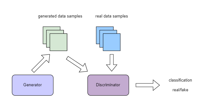
In order to realize the construction of QGANAPI class of quantum generative adversarial network by VQNet, the quantum generator is used to prepare the initial state of the real distributed data. The number of quantum bits is 3, and the repetition times of the internal parametric circuit module of the quantum generator is 1. Meanwhile, KL is used as the metric for the QGAN loading random distribution.

import pickle
import os
import pyqpanda as pq
from pyvqnet.qnn.qgan.qgan_utils import QGANAPI
import numpy as np

num_of_qubits = 3  # paper config
rep = 1
number_of_data = 10000
# Load data samples from different distributions
mu = 1
sigma = 1
real_data = np.random.lognormal(mean=mu, sigma=sigma, size=number_of_data)


# intial
save_dir = None
qgan_model = QGANAPI(
    real_data,
    # numpy generated data distribution, 1 - dim.
    num_of_qubits,
    batch_size=2000,
    num_epochs=2000,
    q_g_cir=None,
    bounds = [0.0,2**num_of_qubits -1],
    reps=rep,
    metric="kl",
    tol_rel_ent=0.01,
    if_save_param_dir=save_dir
)

The following is the train module of QGAN.

# train
qgan_model.train()  # train qgan

The eval module of QGAN is designed to draw the loss function curve and probability distribution diagram between the random distribution prepared by QGAN and the real distribution.

# show probability distribution function of generated distribution and real distribution
qgan_model.eval(real_data)  #draw pdf

The get_trained_quantum_parameters module of QGAN is used to get training parameters and output them as a numpy array. If save_DIR is not empty, the training parameters are saved to a file.The Load_param_and_eval module of QGAN loads training parameters, and the get_circuits_with_trained_param module obtains pyQPanda circuit generated by quantum generator after training.

# get trained quantum parameters
param = qgan_model.get_trained_quantum_parameters()
print(f" trained param {param}")

#load saved parameters files
if save_dir is not None:
    path = os.path.join(
        save_dir, qgan_model._start_time + "trained_qgan_param.pickle")
    with open(path, "rb") as file:
        t3 = pickle.load(file)
    param = t3["quantum_parameters"]
    print(f" trained param {param}")

#show probability distribution function of generated distribution and real distribution
qgan_model.load_param_and_eval(param)

#calculate metric
print(qgan_model.eval_metric(param, "kl"))

#get generator quantum circuit
m_machine = pq.CPUQVM()
m_machine.init_qvm()
qubits = m_machine.qAlloc_many(num_of_qubits)
qpanda_cir = qgan_model.get_circuits_with_trained_param(qubits)
print(qpanda_cir)

In general, QGAN learning and loading random distribution requires multiple training models with different random seeds to obtain the expected results. For example, the following is the graph of the probability distribution function between the lognormal distribution implemented by QGAN and the real lognormal distribution, and the loss function curve between QGAN’s generator and discriminator.

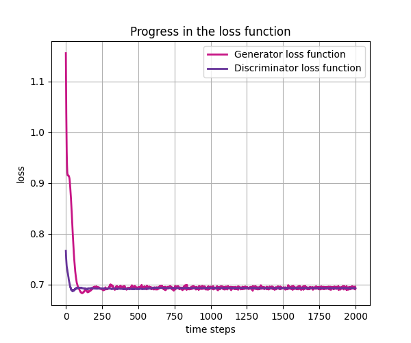
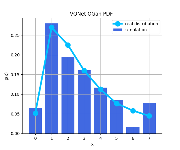
quantum kernal SVM¶

In machine learning tasks, data often cannot be separated by a hyperplane in the original space. A common technique for finding such hyperplanes is to apply a nonlinear transformation function to the data. This function is called a feature map, through which we can calculate how close the data points are in this new feature space for the classification task of machine learning.

This example refers to the thesis: Supervised learning with quantum enhanced feature spaces . The first method constructs variational circuits for data classification tasks.

gen_vqc_qsvm_data is the data needed to generate this example. vqc_qsvm is a variable sub-circuit class used to classify the input data. The vqc_qsvm.plot() function visualizes the distribution of the data.

"""
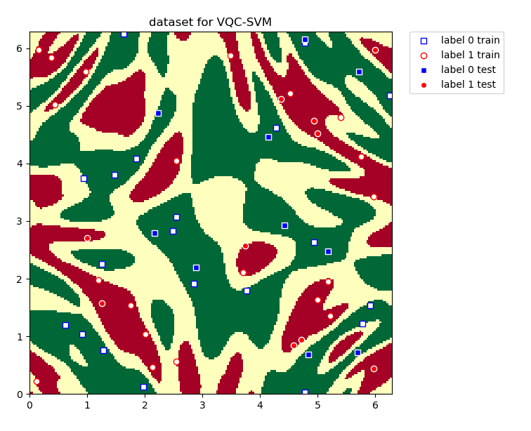
VQC QSVM
"""
from pyvqnet.qnn.svm import vqc_qsvm, gen_vqc_qsvm_data
import matplotlib.pyplot as plt
import numpy as np

batch_size = 40
maxiter = 40
training_size = 20
test_size = 10
gap = 0.3
#sub-circuits repeat times
rep = 3

#defines QSVM class
VQC_QSVM = vqc_qsvm(batch_size, maxiter, rep)
#randomly generates data from thesis.
train_features, test_features, train_labels, test_labels, samples = \
    gen_vqc_qsvm_data(training_size=training_size, test_size=test_size, gap=gap)
VQC_QSVM.plot(train_features, test_features, train_labels, test_labels, samples)
#train
VQC_QSVM.train(train_features, train_labels)
#test
rlt, acc_1 = VQC_QSVM.predict(test_features, test_labels)
print(f"testing_accuracy {acc_1}")

In addition to the above-mentioned direct use of variational quantum circuits to map classical data features to quantum feature spaces, in the paper Supervised learning with quantum enhanced feature spaces, the method of directly estimating kernel functions using quantum circuits and classifying them using classical support vector machines is also introduced. Analogy to various kernel functions in classical SVM \(K(i,j)\) , use quantum kernel function to define the inner product of classical data in quantum feature space \(\phi(\mathbf{x}_i)\) :

\[|\langle \phi(\mathbf{x}_j) | \phi(\mathbf{x}_i) \rangle |^2 = |\langle 0 | U^\dagger(\mathbf{x}_j) U(\mathbf{x}_i) | 0 \rangle |^2\]

Using VQNet and pyQPanda, we define a QuantumKernel_VQNet to generate a quantum kernel function and use sklearn for classification:

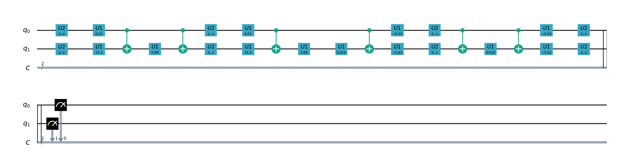
import numpy as np
import pyqpanda as pq
from sklearn.svm import SVC
from pyqpanda import *
from pyqpanda.Visualization.circuit_draw import *
from pyvqnet.qnn.svm import QuantumKernel_VQNet, gen_vqc_qsvm_data
import matplotlib
try:
    matplotlib.use('TkAgg')
except:
    pass
import matplotlib.pyplot as plt

train_features, test_features,train_labels, test_labels, samples = gen_vqc_qsvm_data(20,5,0.3)
quantum_kernel = QuantumKernel_VQNet(n_qbits=2)
quantum_svc = SVC(kernel=quantum_kernel.evaluate)
quantum_svc.fit(train_features, train_labels)
score = quantum_svc.score(test_features, test_labels)
print(f"quantum kernel classification test score: {score}")

Simultaneous Perturbation Stochastic Approximation optimizers¶

pyvqnet.qnn.SPSA(maxiter: int = 1000, save_steps: int = 1, last_avg: int = 1, c0: float = _C0, c1: float = 0.2, c2: float = 0.602, c3: float = 0.101, c4: float = 0, init_para=None, model=None, calibrate_flag=False)¶

Simultaneous Perturbation Stochastic Approximation (SPSA) optimizer.

SPSA provides a stochastic method for approximating the gradient of a multivariate differentiable cost function. To achieve this, the cost function is evaluated twice using a perturbed parameter vector: each component of the original parameter vector is simultaneously shifted by a randomly generated value. Further information is available on the SPSA website.

Parameters:

maxiter – The maximum number of iterations to perform. Default value: 1000.
save_steps – Save the intermediate information of each save_steps step. Default value: 1.
last_avg – Averaging parameter for last_avg iterations. If last_avg = 1, only the last iteration is considered. Default value: 1.
c0 – initial a. Step size for updating parameters. Default value: 0.2*pi
c1 – initial c. The step size used to approximate the gradient. Default: 0.1.
c2 – alpha from the paper, used to adjust a(c0) at each iteration. Default value: 0.602.
c3 – gamma in the paper, used to adjust c(c1) at each iteration. Default value: 0.101.
c4 – Also used to control the parameters of a. Default value: 0.
init_para – Initialization parameters. Default: None.
model – Parametric model: model. Default: None.
calibrate_flag – whether to calibrate hpyer parameters a and c, default value: False.

Returns:

an SPSA optimizer instance

Warning

SPSA only supports 1-dim paramters.

Example:

import numpy as np
import pyqpanda as pq

import sys
sys.path.insert(0, "../")
import pyvqnet

from pyvqnet.nn.module import Module
from pyvqnet.qnn import SPSA
from pyvqnet.tensor.tensor import QTensor
from pyvqnet.qnn import AngleEmbeddingCircuit, expval, QuantumLayerV2, expval
from pyvqnet.qnn.template import BasicEntanglerTemplate

class Model_spsa(Module):
    def __init__(self):
        super(Model_spsa, self).__init__()
        self.qvc = QuantumLayerV2(layer_fn_spsa_pq, 3)

    def forward(self, x):
        y = self.qvc(x)
        return y


def layer_fn_spsa_pq(input, weights):
    num_of_qubits = 1

    machine = pq.CPUQVM()
    machine.init_qvm()
    qubits = machine.qAlloc_many(num_of_qubits)
    c1 = AngleEmbeddingCircuit(input, qubits)
    weights =weights.reshape([4,1])
    bc_class = BasicEntanglerTemplate(weights, 1)
    c2 = bc_class.create_circuit(qubits)
    m_prog = pq.QProg()
    m_prog.insert(c1)
    m_prog.insert(c2)
    pauli_dict = {'Z0': 1}
    exp2 = expval(machine, m_prog, pauli_dict, qubits)

    return exp2

model = Model_spsa()

optimizer = SPSA(maxiter=20,
    init_para=model.parameters(),
    model=model,
)

pyvqnet.qnn.SPSA._step(input_data)¶

use SPSA to optimize input data.

Parameters:

input_data – input data

Returns:

train_para: final parameter

theta_best: The average parameters of after last last_avg.

Example:

import numpy as np
import pyqpanda as pq

import sys
sys.path.insert(0, "../")
import pyvqnet

from pyvqnet.nn.module import Module
from pyvqnet.qnn import SPSA
from pyvqnet.tensor.tensor import QTensor
from pyvqnet.qnn import AngleEmbeddingCircuit, expval, QuantumLayerV2, expval
from pyvqnet.qnn.template import BasicEntanglerTemplate


class Model_spsa(Module):
    def __init__(self):
        super(Model_spsa, self).__init__()
        self.qvc = QuantumLayerV2(layer_fn_spsa_pq, 3)

    def forward(self, x):
        y = self.qvc(x)
        return y


def layer_fn_spsa_pq(input, weights):
    num_of_qubits = 1

    machine = pq.CPUQVM()
    machine.init_qvm()
    qubits = machine.qAlloc_many(num_of_qubits)
    c1 = AngleEmbeddingCircuit(input, qubits)
    weights =weights.reshape([4,1])
    bc_class = BasicEntanglerTemplate(weights, 1)
    c2 = bc_class.create_circuit(qubits)
    m_prog = pq.QProg()
    m_prog.insert(c1)
    m_prog.insert(c2)
    pauli_dict = {'Z0': 1}
    exp2 = expval(machine, m_prog, pauli_dict, qubits)

    return exp2

model = Model_spsa()

optimizer = SPSA(maxiter=20,
    init_para=model.parameters(),
    model=model,
)

data = QTensor(np.array([[0.27507603]]))
p = model.parameters()
p[0].data = pyvqnet._core.Tensor( np.array([3.97507603, 3.12950603, 1.00854038,
                1.25907603]))

optimizer._step(input_data=data)


y = model(data)
print(y)

Quantum fisher information computation matrix¶

class pyvqnet.qnn.opt.quantum_fisher(py_qpanda_config, params, target_gate_type_lists, target_gate_bits_lists, qcir_lists, wires)¶

Returns the quantum fisher information matrix for a quantum circuit.

\[\mathrm{QFIM}_{i, j}=4 \operatorname{Re}\left[\left\langle\partial_i \psi(\boldsymbol{\theta}) \mid \partial_j \psi(\boldsymbol{\theta})\right\rangle-\left\langle\partial_i \psi(\boldsymbol{\theta}) \mid \psi(\boldsymbol{\theta})\right\rangle\left\langle\psi(\boldsymbol{\theta}) \mid \partial_j \psi(\boldsymbol{\theta})\right\rangle\right]\]

The short version is :math:\(\left|\partial_j \psi(\boldsymbol{\theta})\right\rangle:=\frac{\partial}{\partial \theta_j}|\psi(\boldsymbol{\theta})\rangle\).

Note

Currently only RX,RY,RZ are supported.

Parameters:

params – Variable parameters in circuits.
target_gate_type_lists – Supports “RX”, “RY”, “RZ” or lists.
target_gate_bits_lists – Which quantum bit or bits the parameterised gate acts on .
qcir_lists – The list of quantum circles before the target parameterised gate to compute the metric tensor, see the following example.
wires – Total Quantum Bit Index for Quantum Circuits.

Example:

import pyqpanda as pq

from pyvqnet import *
from pyvqnet.qnn.opt import pyqpanda_config_wrapper, insert_pauli_for_mt, quantum_fisher
from pyvqnet.qnn import ProbsMeasure
import numpy as np
import pennylane as qml
import pennylane.numpy as pnp

n_wires = 4
def layer_subcircuit_new(config: pyqpanda_config_wrapper, params):
    qcir = pq.QCircuit()
    qcir.insert(pq.RX(config._qubits[0], params[0]))
    qcir.insert(pq.RY(config._qubits[1], params[1]))

    qcir.insert(pq.CNOT(config._qubits[0], config._qubits[1]))

    qcir.insert(pq.RZ(config._qubits[2], params[2]))
    qcir.insert(pq.RZ(config._qubits[3], params[3]))
    return qcir


def get_p1_diagonal_new(config, params, target_gate_type, target_gate_bits,
                    wires):
    qcir = layer_subcircuit_new(config, params)
    qcir2 = insert_pauli_for_mt(config._qubits, target_gate_type,
                                target_gate_bits)
    qcir3 = pq.QCircuit()
    qcir3.insert(qcir)
    qcir3.insert(qcir2)

    m_prog = pq.QProg()
    m_prog.insert(qcir3)
    return ProbsMeasure(wires, m_prog, config._machine, config._qubits)

config = pyqpanda_config_wrapper(n_wires)
qcir = []

qcir.append(get_p1_diagonal_new)

params2 = QTensor([0.5, 0.5, 0.5, 0.25], requires_grad=True)

mt = quantum_fisher(config, params2, [['RX', 'RY', 'RZ', 'RZ']],
                        [[0, 1, 2, 3]], qcir, [0, 1, 2, 3])

# The above example shows that there are no identical gates in the same layer,
# but in the same layer you need to modify the logic gates according to the following example.

n_wires = 3
def layer_subcircuit_01(config: pyqpanda_config_wrapper, params):
    qcir = pq.QCircuit()
    qcir.insert(pq.RX(config._qubits[0], params[0]))
    qcir.insert(pq.RY(config._qubits[1], params[1]))
    qcir.insert(pq.CNOT(config._qubits[0], config._qubits[1]))

    return qcir

def layer_subcircuit_02(config: pyqpanda_config_wrapper, params):
    qcir = pq.QCircuit()
    qcir.insert(pq.RX(config._qubits[0], params[0]))
    qcir.insert(pq.RY(config._qubits[1], params[1]))
    qcir.insert(pq.CNOT(config._qubits[0], config._qubits[1]))
    qcir.insert(pq.RZ(config._qubits[1], params[2]))
    return qcir

def layer_subcircuit_03(config: pyqpanda_config_wrapper, params):
    qcir = pq.QCircuit()
    qcir.insert(pq.RX(config._qubits[0], params[0]))
    qcir.insert(pq.RY(config._qubits[1], params[1]))
    qcir.insert(pq.CNOT(config._qubits[0], config._qubits[1])) #  01 part

    qcir.insert(pq.RZ(config._qubits[1], params[2]))  #  02 part

    qcir.insert(pq.RZ(config._qubits[1], params[3]))
    return qcir

def get_p1_diagonal_01(config, params, target_gate_type, target_gate_bits,
                    wires):
    qcir = layer_subcircuit_01(config, params)
    qcir2 = insert_pauli_for_mt(config._qubits, target_gate_type,
                                target_gate_bits)
    qcir3 = pq.QCircuit()
    qcir3.insert(qcir)
    qcir3.insert(qcir2)

    m_prog = pq.QProg()
    m_prog.insert(qcir3)
    return ProbsMeasure(wires, m_prog, config._machine, config._qubits)

def get_p1_diagonal_02(config, params, target_gate_type, target_gate_bits,
                    wires):
    qcir = layer_subcircuit_02(config, params)
    qcir2 = insert_pauli_for_mt(config._qubits, target_gate_type,
                                target_gate_bits)
    qcir3 = pq.QCircuit()
    qcir3.insert(qcir)
    qcir3.insert(qcir2)

    m_prog = pq.QProg()
    m_prog.insert(qcir3)
    return ProbsMeasure(wires, m_prog, config._machine, config._qubits)

def get_p1_diagonal_03(config, params, target_gate_type, target_gate_bits,
                    wires):
    qcir = layer_subcircuit_03(config, params)
    qcir2 = insert_pauli_for_mt(config._qubits, target_gate_type,
                                target_gate_bits)
    qcir3 = pq.QCircuit()
    qcir3.insert(qcir)
    qcir3.insert(qcir2)

    m_prog = pq.QProg()
    m_prog.insert(qcir3)
    return ProbsMeasure(wires, m_prog, config._machine, config._qubits)

config = pyqpanda_config_wrapper(n_wires)
qcir = []

qcir.append(get_p1_diagonal_01)
qcir.append(get_p1_diagonal_02)
qcir.append(get_p1_diagonal_03)

params2 = QTensor([0.5, 0.5, 0.5, 0.25], requires_grad=True)

mt = quantum_fisher(config, params2, [['RX', 'RY'], ['RZ'], ['RZ']], # rx,ry counts as layer one, first rz as layer two, second rz as layer three.
                        [[0, 1], [1], [1]], qcir, [0, 1])