Steps of VQNet Installation
VQNet python package Installation
We provide precompiled Python packages for installation on Linux, Windows, macOS 13+ (arm64), supporting Python 3.10.
Download the corresponding archive from the official website, extract it, navigate to the extracted directory, and run the following steps:
# For Windows
./install.batch
# For macOS and Linux
./install.sh
For Windows and Linux systems, the pyvqnet package includes built-in acceleration features for classic neural network computations based on Nvidia CUDA, which depends on the specific version of NVIDIA CUDA 12.6 runtime libraries (automatically installed with the package). The package is optimized for the following CUDA architectures: sm_80 (NVIDIA A100, A30 series data center GPUs) and sm_86 (NVIDIA GeForce RTX 30 series consumer GPUs). Please ensure you are using a GPU that supports these architectures; otherwise, the program may not function correctly.
Important
Please note that since this package does not distinguish between CPU/GPU versions, it depends on NVIDIA CUDA runtime libraries under Windows and Linux, which are automatically installed with the package. This may cause conflicts with other software that depends on different versions.
Validate VQNet’s installation
import pyvqnet
from pyvqnet.tensor import *
a = arange(1,25).reshape([2, 3, 4])
print(a)
Testing GPU Functionality in VQNet
from pyvqnet import DEV_GPU_0
from pyvqnet.tensor import *
a = ones([4,5],device = DEV_GPU_0)
print(a)
A simple case of VQNet
Here we introduce a case that consists of classical neural network modules and quantum modules of VQNet to describe the workflow of quantum machine learning. It refers to Data re-uploading for a universal quantum classifier . Generally, there are the following parts of quantum computing module in quantum machine learning:
(1)Encoder:encoding classical data into quantum state;
(2)Ansats: training the parameters in Parameterized Quantum Gates;
(3)Measurement: measuring the value of a qubit(projection of qubit’s quantum state in a specified axis).
Quantum computing module is the theoretical basis of the hybrid model of quantum classical neural network, which is also differentiable like classical neural network modules. VQNet supports quantum computing modules and classical computing modules to form a hybrid machine learning model, and provides various optimization algorithms for parameter optimization. (e.g. Convolution layer, pooling layer, fully connected layer, activation function, etc.)
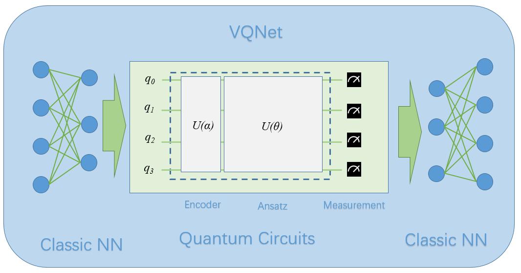
In the quantum computing module, VQNet supports the use of the efficient quantum software computing package pyqpanda3 to build quantum modules. Using the various commonly used interfaces provided by pyqpanda3, users can quickly build quantum computing modules.
The following example uses pyqpanda3 to build a quantum computing module. Through VQNet, this quantum module can be directly embedded into a hybrid machine learning model for quantum circuit parameter training. In this example, 1 qubit is used, multiple parameterized rotation gates RZ, RY, RZ are used to encode the input x, and the probs_measure function is used to observe the probability measurement result of the qubit as output.
import pyqpanda3.core as pq
from pyvqnet.qnn.pq3 import probs_measure
def qdrl_circuit(input,weights):
    qlist = range(1)
    machine = pq.CPUQVM()
    x1 = input.squeeze()
    param1 = weights.squeeze()
    # Build quantum circuit instance using pyqpanda3 interface
    circuit = pq.QCircuit()
    # Insert RZ gate on the first qubit with parameter x1[0]
    circuit << pq.RZ(qlist[0], x1[0])
    # Insert RY gate on the first qubit with parameter x1[1]
    circuit << pq.RY(qlist[0], x1[1])
    # Insert RZ gate on the first qubit with parameter x1[2]
    circuit << pq.RZ(qlist[0], x1[2])
    # Insert RZ gate on the first qubit with parameter param1[0]
    circuit << pq.RZ(qlist[0], param1[0])
    # Insert RY gate on the first qubit with parameter param1[1]
    circuit << pq.RY(qlist[0], param1[1])
    # Insert RZ gate on the first qubit with parameter param1[2]
    circuit << pq.RZ(qlist[0], param1[2])
    # Insert RZ gate on the first qubit with parameter x1[0]
    circuit << pq.RZ(qlist[0], x1[0])
    # Insert RY gate on the first qubit with parameter x1[1]
    circuit << pq.RY(qlist[0], x1[1])
    # Insert RZ gate on the first qubit with parameter x1[2]
    circuit << pq.RZ(qlist[0], x1[2])
    # Insert RZ gate on the first qubit with parameter param1[3]
    circuit << pq.RZ(qlist[0], param1[3])
    # Insert RY gate on the first qubit with parameter param1[4]
    circuit << pq.RY(qlist[0], param1[4])
    # Insert RZ gate on the first qubit with parameter param1[5]
    circuit << pq.RZ(qlist[0], param1[5])
    # Insert RZ gate on the first qubit with parameter x1[0]
    circuit << pq.RZ(qlist[0], x1[0])
    # Insert RY gate on the first qubit with parameter x1[1]
    circuit << pq.RY(qlist[0], x1[1])
    # Insert RZ gate on the first qubit with parameter x1[2]
    circuit << pq.RZ(qlist[0], x1[2])
    # Insert RZ gate on the first qubit with parameter param1[6]
    circuit << pq.RZ(qlist[0], param1[6])
    # Insert RY gate on the first qubit with parameter param1[7]
    circuit << pq.RY(qlist[0], param1[7])
    # Insert RZ gate on the first qubit with parameter param1[8]
    circuit << pq.RZ(qlist[0], param1[8])
    # Build quantum program
    prog = pq.QProg()
    prog << circuit
    # Get probability measurement
    prob = probs_measure(machine ,prog,  qlist)

    return prob
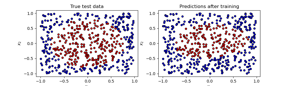
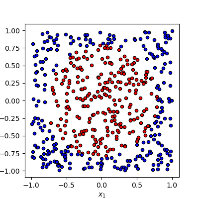
Our task is to classify this randomly generated data using a binary classification approach. In this task, the center of a circle is at the origin, points within radius 1 colored in red belong to one category, and the samples colored in blue belong to another category.
The pipeline of the training process
# import required libraries and functions
from pyvqnet.qnn.pq3.quantumlayer import QuantumLayer
from pyvqnet.optim import adam
from pyvqnet.nn.loss import CategoricalCrossEntropy
from pyvqnet.tensor import QTensor
import numpy as np
from pyvqnet.nn.module import Module
Defining a model: the __init__ function defines the internal neural network modules and quantum modules, and the forward function defines the forward computation. QuantumLayer is an abstract class
that encapsulates quantum computing.
VQNet will automatically calculate the parameter gradients for qdrl_circuit with param_num.
# number of parameters to be trained.
param_num = 9
# qubit number.
qbit_num  = 1
#define a model class inherits from Module.
class Model(Module):
    def __init__(self):
        super(Model, self).__init__()
        #use QuantumLayer to embed quantum circuit into autodiff pipeline.
        self.pqc = QuantumLayer(qdrl_circuit,param_num)
    #define the forward function
    def forward(self, x):
        x = self.pqc(x)
        return x
Defining some functions for training the model
# a function to generate the raw data randomly
def circle(samples:int,  rads =  np.sqrt(2/np.pi)) :
    data_x, data_y = [], []
    for i in range(samples):
        x = 2*np.random.rand(2) - 1
        y = [0,1]
        if np.linalg.norm(x) < rads:
            y = [1,0]
        data_x.append(x)
        data_y.append(y)
    return np.array(data_x,dtype=np.float32), np.array(data_y,np.int64)

# a function to load data
def get_minibatch_data(x_data, label, batch_size):
    for i in range(0,x_data.shape[0]-batch_size+1,batch_size):
        idxs = slice(i, i + batch_size)
        yield x_data[idxs], label[idxs]

# a function to compute the accuracy
def get_score(pred, label):
    pred, label = np.array(pred.data), np.array(label.data)
    pred = np.argmax(pred,axis=1)
    score = np.argmax(label,1)
    score = np.sum(pred == score)
    return score
VQNet follows the general workflow of machine learning: loading the data iteratively, forward propagation, calculating the loss function, back propagation, and updating the parameters.
# instantiating a model
model = Model()
# using Adam to define a optimizer
optimizer = adam.Adam(model.parameters(),lr =0.6)
# using cross-entropy to define a loss function
Closs = CategoricalCrossEntropy()
A function to train the model
def train():

    #  generate data to be trained randomly
    x_train, y_train = circle(500)
    x_train = np.hstack((x_train, np.zeros((x_train.shape[0], 1),dtype=np.float32)))
    # define the number of data about each batch
    batch_size = 32
    # Maximum of training iteration times
    epoch = 10
    print("start training...........")
    for i in range(epoch):
        model.train()
        accuracy = 0
        count = 0
        loss = 0
        for data, label in get_minibatch_data(x_train, y_train,batch_size):
            # clear the gradients of optimizer
            optimizer.zero_grad()
            # forward computing
            output = model(data)
            # calculating loss function
            losss = Closs(label, output)
            # anti-propagation
            losss.backward()
            # update the optimizer parameters
            optimizer._step()
            # calculate the accuracy
            accuracy += get_score(output,label)

            loss += losss.item()
            count += batch_size

        print(f"epoch:{i}, train_accuracy:{accuracy/count}")
        print(f"epoch:{i}, train_loss:{loss/count}\n")
A function to validate the model
def test():

    batch_size = 1
    model.eval()
    print("start eval...................")
    xtest, y_test = circle(500)
    test_accuracy = 0
    count = 0
    x_test = np.hstack((xtest, np.zeros((xtest.shape[0], 1),dtype=np.float32)))

    for test_data, test_label in get_minibatch_data(x_test,y_test, batch_size):

        test_data, test_label = QTensor(test_data),QTensor(test_label)
        output = model(test_data)
        test_accuracy += get_score(output, test_label)
        count += batch_size

    print(f"test_accuracy:{test_accuracy/count}")
Training and testing results
start training...........
epoch:0, train_accuracy:0.6145833333333334
epoch:0, train_loss:0.020432369535168013

epoch:1, train_accuracy:0.6854166666666667
epoch:1, train_loss:0.01872217481335004

epoch:2, train_accuracy:0.8104166666666667
epoch:2, train_loss:0.016634768371780715

epoch:3, train_accuracy:0.7479166666666667
epoch:3, train_loss:0.016975031544764835

epoch:4, train_accuracy:0.7875
epoch:4, train_loss:0.016502128106852372

epoch:5, train_accuracy:0.8083333333333333
epoch:5, train_loss:0.0163204787299037

epoch:6, train_accuracy:0.8083333333333333
epoch:6, train_loss:0.01634311651190122

epoch:7, train_loss:0.016330583145221074

epoch:8, train_accuracy:0.8125
epoch:8, train_loss:0.01629052646458149

epoch:9, train_accuracy:0.8083333333333333
epoch:9, train_loss:0.016270687493185203

start eval...................
test_accuracy:0.826